Bayesian statistics updates a probability when new evidence arrives. Start with a prior: the best estimate with little information. Treat the new information as an event, then calculate a posterior: the refined estimate after taking that event into account. section 8.2 section 8.0
A positive test is not the whole story
Suppose a rare disease affects 1 in 10,000 people and a test is 99% accurate. Among one million people, about 100 are sick. A positive result identifies 99 sick people, but also 9,999 healthy people incorrectly. Given a positive test, the chance of actually being sick is about 0.0098—not 99%. The low prior probability matters. section 8.1 section 8.2
Figure 8.1 Among our 1,000,000 patients, only 100 of them are sick (bottom row). Among the 10,098 diagnosed as sick (left column), only 99 of them are actually sick. The remaining 9,999 are healthy, yet were misdiagnosed as sick. Therefore, if our friend was diagnosed as sick, he has a much higher chance to be among the 9,999 healthy (top left) than to be among the 99 sick (bottom left).
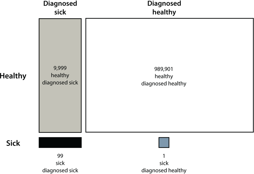
Use the patient-count table to see why false positives can outnumber true positives when the condition is rare. section 8.1
Bayes’ theorem answers a conditional question: “What is the probability of Y, given that X happened?” In plain language, compare each possible explanation for the evidence, then normalize the resulting probabilities so they add up to one. This turns an initial guess into an evidence-aware estimate. section 8.0 section 8.6
Does “lottery” suggest spam?
If 20 of 100 emails contain “lottery,” and 15 of those 20 are spam, then the posterior probability of spam given “lottery” is 15/20, or 0.75. The overall spam rate is the prior; seeing the word changes that estimate. section 8.5 section 8.6
Naive Bayes applies this update to several events, such as the words in an email. It assumes those events are independent, multiplies their class-specific probabilities, and uses Bayes’ theorem to produce probabilities for spam and ham. Word counts can estimate those probabilities; initializing counts at 1 avoids zero-count divisions. section 8.15 section 8.12 section 8.8
A small spam predictor
A Python predictor lowercases an email, examines known words, and combines their spam and ham probabilities. “Hi mom how are you” receives about 0.12 spam probability, while “buy cheap lottery easy money now” receives over 0.99. An email with no known words falls back to the prior. section 8.13