Categorical data represents a variable that takes one value from a finite set of allowed categories rather than any value on a continuous numerical range. A binary variable is the special case with exactly two categories, such as 0 = do not sell and 1 = sell. section 7.2
In machine learning, a categorical output defines a classification problem: a function maps an input to one class. A face detector, for example, maps an image represented as a point in a high-dimensional input space to 0 (not face) or 1 (face). section 7.2.2
Geometrically, classification partitions the input space into regions associated with different categories. The boundary may be linear, as with a perceptron, or may approximate a more complex true boundary; the input variables themselves may be continuous or categorical. section 7.2.2
Binary face classification
Given an image vector x, a classifier produces a categorical output ϕ(x) ∈ {0, 1}. The value 0 denotes no face, while 1 denotes a face. This categorical decision differs from estimating the probability that the image contains a face, which produces a continuous output. section 7.2.2 section 7.2.3
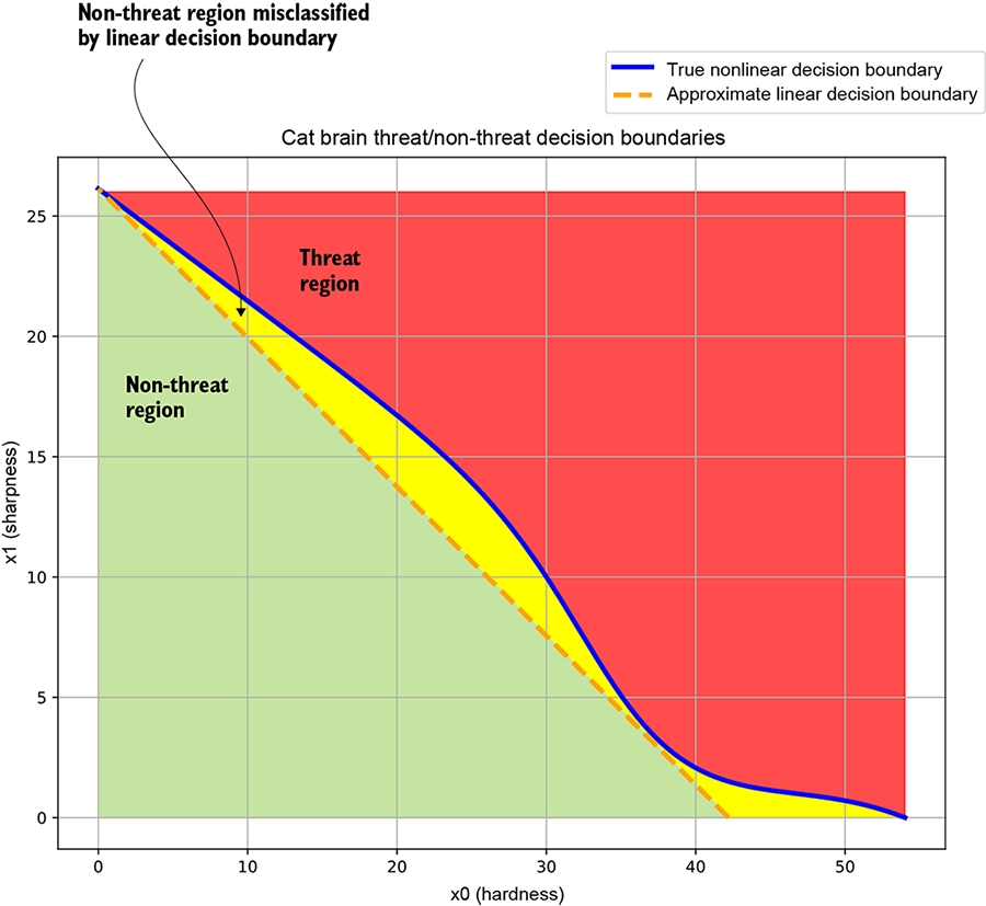
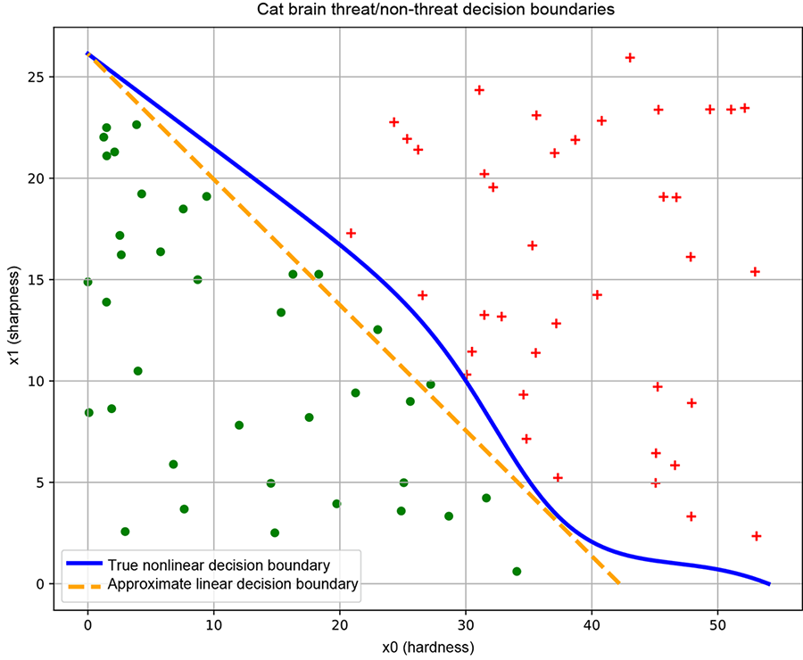
Figure 7.4 Classifiers, decision boundaries, and training data. Data points from different classes are marked with different symbols (plus and dot).
|
(a) Cat brain threat model decision boundary. The solid curve corresponds to the true decision boundary separating the threat and non-threat regions. The dashed line represents an approximate linear decision boundary: it classifies most points correctly but misclassifies points in the region between itself and the true decision boundary. |
|
(b) Good training data. Sample points from each class roughly span the region of input space belonging to the class. This yields a good decision boundary (solid line). |
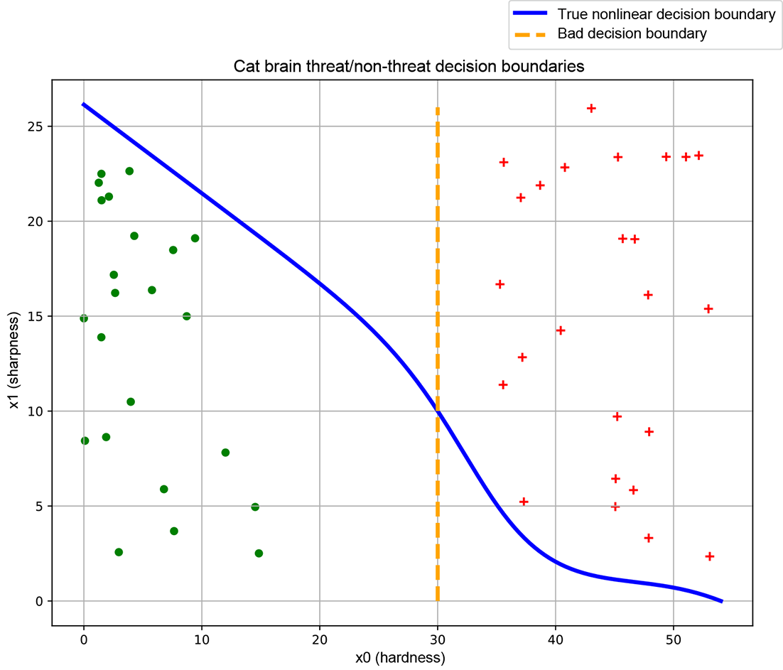
Compare how training samples from different categories cover input-space regions and how that coverage affects the resulting decision boundary. section 7.2.2