Hidden layer

As explained in Grokking AI Algorithms, Second Edition

A hidden layer is an intermediate computational layer in a neural network whose units receive inputs from preceding layers and pass transformed values to subsequent layers.

A hidden layer sits between a neural network’s inputs and outputs. It is “hidden” because people provide inputs and see predictions, but do not directly observe the intermediate values. Each node combines its inputs using weights, then applies an activation function. The resulting values pass to the next layer. section 9.3 section 9.23

Estimating a collision

Imagine predicting whether a car collision will occur from speed, terrain quality, degree of vision, and driving experience. First, scale the four inputs. Then each hidden node calculates a weighted sum and applies an activation function such as sigmoid. One node might give terrain and vision stronger weights than speed and experience, making it especially responsive to their relationship. Finally, the output node combines the hidden nodes’ results to produce a prediction. The nodes work together; none needs to make the whole decision alone. section 9.3 section 9.4

Figure 9.12 Example of a hidden node comparing terrain quality and degree of vision

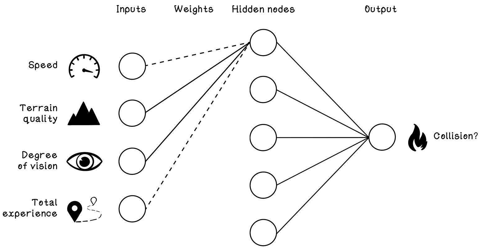
See how stronger connections can make one hidden node respond chiefly to terrain quality and degree of vision. section 9.3

The calculation need not run node by node. Put the four inputs in a vector and the weights for five hidden nodes in a 4 × 5 matrix. One matrix multiplication gives all five weighted sums; applying the activation function gives the layer’s output. A learning-oriented Python implementation expresses this as `hidden = sigmoid(np.dot(inputs, input_weights))`, then passes `hidden` through another weighted, activated layer. section 9.21 section 9.4

More hidden layers can capture higher-level relationships and more complex classification boundaries, but there is no universally ideal count of layers or nodes. Choose an architecture by considering the data and testing changes. During training, backpropagation traces how weights inside hidden layers affect the prediction and its error, so those weights can be adjusted. section 9.13 section 9.26

How Grokking AI Algorithms, Second Edition covers it

How deep it goes

Works through weighted sums, activations, matrix multiplication, and a forward-pass implementation, while treating layer and node counts as experimental choices.

Examples

Traces car-collision features through five hidden nodes and illustrates a node weighted toward terrain quality and degree of vision.

What it assumes

Introduces hidden nodes through input features and output labels, then breaks down weighted sums and activation during forward propagation.

What you can do after

Build it from scratch with NumPy matrix operations and sigmoid activation, then experiment with the number of hidden nodes and layers.

How it connects

Connects hidden layers to activation functions, forward propagation, backpropagation, tensors, and recurrent neural networks.

liveBookmanning.com

Read Grokking AI Algorithms, Second Edition on liveBook Get the book at manning.com

Also explained in

• 

  liveBookmanning.com
  Grokking Machine LearningA neural-network layer positioned between the input and output layers whose units transform intermediate representations.
• 

  liveBookmanning.com
  Classic Computer Science Problems in Swift: Essential techniques for practicing programmersA hidden layer is a neural-network layer between the input and output layers whose outputs are not the network's final outputs.
• 

  liveBookmanning.com
  Inside AIA hidden layer is an intermediate neural-network layer that transforms representations between the input and output layers.
• 

  liveBookmanning.com
  Graph Neural Networks in ActionAn intermediate layer of a neural network whose activations are not directly exposed as the model's inputs or outputs.
• 

  liveBookmanning.com
  Natural Language Processing in Action, Second EditionA hidden layer is an intermediate neural-network layer whose activations are not directly exposed as the model's input or final output.
• 

  liveBookmanning.com
  Inside Deep Learning: Math, Algorithms, ModelsA network layer between input and output that transforms representations before later computation, here before attention is applied.
• 

  liveBookmanning.com
  Data Without LabelsA hidden layer is an intermediate neural-network layer whose activations are not directly observed as inputs or outputs.

Compare how 8 books explain hidden layer →

Related concepts

• neural network layerkind of · A neural network layer is a computational stage or component that transforms input representations into outputs within a neural network.
• deep learningpart of · Deep learning is a machine-learning approach that uses neural networks with multiple computational layers to learn representations from data.
• language modelpart of · A language model is a computational model that represents patterns in linguistic tokens to estimate sequence probabilities and predict or generate language from context.
• neural networkpart of · A neural network is a computational model of interconnected, parameterized units that learns transformations from inputs to outputs.
• recurrent neural networkpart of · A recurrent neural network is a neural network that processes sequences by updating an internal state across successive inputs, allowing earlier inputs to influence later computations.
• dropoutused by · Dropout is a neural-network regularization technique that randomly suppresses units, connections, or activations during training to reduce overfitting.

This explainer was generated by Manning's knowledge graph from the text of Grokking AI Algorithms, Second Edition. The section links point to the parts of the book it draws on.