Drift is a change in a time series’ statistical behavior over time. A series whose mean, variance, or autocovariance does not remain constant is nonstationary. Trends, seasonal fluctuations, and abrupt market shifts can all complicate forecasting; stock closing prices are a practical example. Do not assume that every observed change follows a stable pattern a model can extrapolate. section 7.3.6 section 7.2
Check for nonstationarity before fitting a model that assumes stationary data:
- Split observations in time order. Fit and preprocess using the training period, leaving later observations for a forecasting check. section 7.3.7
- Inspect the training series for trends or seasonality, then examine its autocorrelation function (ACF) and partial autocorrelation function (PACF) for lagged relationships. section 7.3.7
- Apply a stationarity test rather than relying on appearance alone. In the closing-price example, the original training series produces an augmented Dickey–Fuller (ADF) p-value of 0.5761116196186049. section 7.3.7
Remove a changing level with first-order differencing
Subtract each preceding value from the current value: 171.953735 − 173.300247 = −1.346512. Five closing prices yield four differences because the first price has no predecessor. In Python, `train_diff = train.diff().dropna()` performs this transformation on the training set. Compare the original and differenced plots and lag correlations, then test again: the differenced example produces an ADF p-value of 1.2486140415792743e-16. First-order differencing addresses a changing level; seasonal differencing is another option when periodic fluctuations are the issue. Verify the result rather than presuming that differencing always resolves nonstationarity. section 7.3.6 section 7.3.7
Figure 7.6 ACF and PACF plots for the original time series (top row) and first-order differenced time series (bottom row). The left column displays the ACF, showing how each observation is correlated with its previous values, whereas the right column presents the PACF, illustrating the direct effect of each lag. These plots are provided to compare the effect of first-order differencing on the time series’ correlation structure.
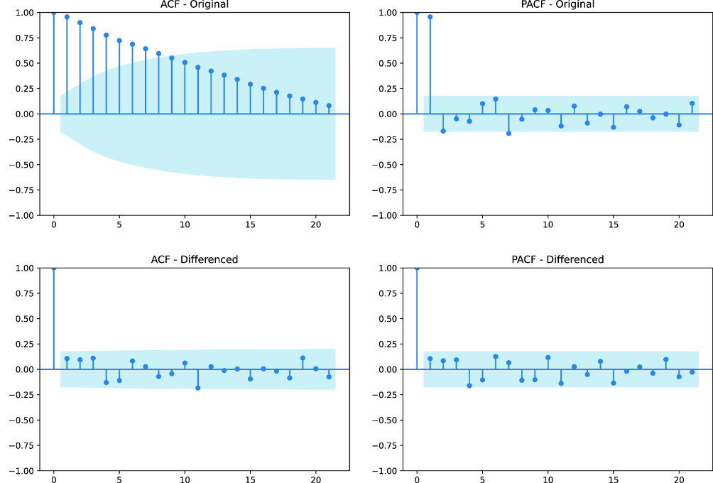
Compare ACF and PACF plots before and after differencing to see how the training series’ lag-correlation structure changes. section 7.3.7