Regression coefficient

As explained in Statistics Every Programmer Needs

A regression coefficient is a parameter quantifying the modeled relationship between a predictor and a response, conditional on the other model terms.

A regression coefficient estimates how a predictor relates to a response. In linear regression, a predictor’s coefficient gives the expected change in the numeric response for a one-unit increase in that predictor; its sign gives the direction of the relationship. In multiple regression, interpret that change with the other model terms held fixed. section 4.0 section 4.2.3 section 5.1

For a simple linear regression, write the prediction as ŷ = a + bx. The slope b equals Σ(x − x̄)(y − ȳ) / Σ(x − x̄)²; the intercept a equals ȳ − bx̄ and gives the predicted response at x = 0. These estimates define the fitted line, but they do not establish by themselves that its predictions are reliable. section 4.2.3 section 4.0

Predict a race split time

A fitted model predicts Stage 2 running time from Stage 1 time: ŷ = −3.078 + 1.3083x, with times in minutes. For x = 193, Python’s round(-3.078 + 1.3083 * 193) gives 249 minutes. The positive slope associates a one-minute longer Stage 1 time with about 1.31 additional predicted Stage 2 minutes. The reported R² is about 0.575; evaluate fit and assumptions before relying on the prediction. section 4.2.3 section 4.0

Figure 4.5 A scatter plot that displays the observed stage1 and stage2 values from the mds data frame, their respective x and y coordinates, and a regression line that represents the predictions for stage2 from a simple linear regression where stage2 was regressed against stage1. The regression line is drawn by applying the linear equation at the top of the plot. R-squared is one of several metrics contained in the model output; it represents the percentage of variance in stage2 that can be explained by changes in stage1.

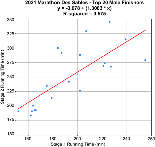
The observed race times and fitted line show what the coefficients predict—and how observations vary around those predictions. section 4.2.3

In logistic regression, coefficients have a different scale: a one-unit predictor change corresponds to a change in the log odds of a binary outcome, not a direct change in its probability. The predictors and coefficients form the input to a sigmoid function, which produces a probability between 0 and 1. For either model, consider statistical significance, collinearity and model assumptions alongside coefficient size. section 5.1 section 4.0

How Statistics Every Programmer Needs covers it

How deep it goes

Works through linear slope and intercept calculations and a prediction; contrasts logistic log-odds coefficients with linear response changes.

Examples

Uses race-stage split times, a fitted regression line and a 193-minute input yielding a 249-minute prediction.

What it assumes

Assumes predictor and response variables are identifiable; develops simple-regression estimates from observed values and their means.

What you can do after

Apply it via a fitted linear equation to predict a response, then assess fit and assumptions before interpreting the estimate.

How it connects

Connects linear regression, logistic regression, intercepts, log odds, sigmoid functions, statistical significance and collinearity.

liveBookmanning.com

Read Statistics Every Programmer Needs on liveBook Get the book at manning.com

Also explained in

• 

  liveBookmanning.com
  Machine Learning for Tabular Data: XGBoost, Deep Learning, and AIA regression coefficient is a parameter multiplying an input variable that determines its signed contribution to a linear regression model's prediction.
• 

  liveBookmanning.com
  Starting Data Analytics with Generative AI and PythonA regression coefficient is an estimated parameter expressing the change in a modeled outcome associated with a one-unit change in a predictor while other predictors are held constant.
• 

  liveBookmanning.com
  Causal Inference for Data ScienceA regression coefficient is a parameter quantifying the change in a modeled outcome associated with a one-unit change in a predictor while other predictors are held fixed.
• 

  liveBookmanning.com
  Statistics Slam DunkA regression coefficient is a fitted parameter quantifying the change in a response associated with a one-unit change in a predictor while other predictors are held constant.

Compare how 5 books explain regression coefficient →

Related concepts

• logitmeasures · A logit is a real-valued quantity representing an outcome’s log-odds or, in machine learning, an unnormalized model score used to derive probabilities.
• parameterkind of · A model parameter is a numerical value, such as a weight or bias, that is learned or set to determine how a model computes outputs.
• linear regressionproduced by · Linear regression is a statistical modeling method that estimates a continuous response as a linear combination of predictor variables and fitted coefficients.
• maximum likelihood estimationproduced by · Maximum likelihood estimation is a statistical method that selects parameter values maximizing the likelihood of observed data under a specified probabilistic model.
• treatment effectcontrasts with · A treatment effect is the difference in an outcome attributable to receiving an intervention or exposure rather than a comparison condition.
• direct effectequivalent to · A direct effect is the portion of a causal effect transmitted along a specified direct causal path from a cause to an outcome, excluding effects through mediators.

This explainer was generated by Manning's knowledge graph from the text of Statistics Every Programmer Needs. The section links point to the parts of the book it draws on.