A slope is the regression coefficient that measures the expected change in a dependent variable for each one-unit increase in a predictor. In simple linear regression, β1 is the slope in ŷ = β0 + β1x; β0 is the intercept, and ŷ is the predicted response. section 4.1.1
Use the slope to interpret the direction, magnitude, and predictive line of a fitted regression:
- A positive slope means the response tends to increase as the predictor increases; a negative slope means the variables move in opposite directions. section 4.1.1
- In multiple regression, each predictor has its own slope coefficient, representing its contribution within the fitted equation. section 4.1.1
- Estimate the slope from centered values as the sum of (x − x̅)(y − ȳ) divided by the sum of (x − x̅)². section 4.2.3
- Interpret the coefficient alongside predictive power and statistical significance rather than treating it as a complete model evaluation. section 4.2.3
Predicting a marathon split
A fitted regression for Stage 2 time from Stage 1 time has intercept −3.0778 and slope 1.3083: ŷ = −3.0778 + 1.3083x. For a Stage 1 split of 193 minutes, the predicted Stage 2 split is approximately 249 minutes. Python can draw the fitted line with `yhat = -3.078 + (1.3083 * x)` and overlay it on a Matplotlib scatter plot. section 4.2.3
Figure 4.1 A scatter plot that displays eight data points, their respective x and y coordinates, and a regression line. The data points represent the observed data (for instance, when x equals 202, y equals 288, which has been highlighted and magnified). The regression line ties back to a simple linear regression that was fit on the data, where a response variable called y, which runs along the y axis, was regressed against a predictor called x, which runs along the x axis. It represents the linear equation at the top that can be derived from the model output, which is to say, it is also a representation of the predictions for y given x. R-squared is one of several metrics contained in the model output; it represents the percentage of variance in the response variable that can be explained by changes in the predictor.
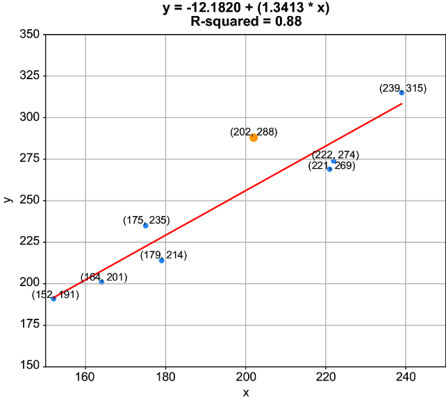
Inspect the observed points, their coordinates, and the fitted regression line to connect the slope with predicted responses. section 4.1.1