Standard deviation measures how widely values in a probability distribution spread around its mean. It is nonnegative and equals the square root of the variance, so a larger value indicates a broader distribution and greater uncertainty. section 3.12 section 13.3
For a normal distribution, the mean μ describes the center and the standard deviation σ describes the spread. The notation N(μ, σ²) uses variance, σ², to emphasize that spread cannot be negative. Roughly 95% of normally distributed values lie between μ − 2σ and μ + 2σ; more precisely, the 95% interval is μ ± 1.96σ. section 3.12
A wide prior expresses uncertainty
A prior for a price-per-square-foot slope can use μ = 100 and σ = 100. Its center is $100, while its large standard deviation produces a broad distribution: approximately 95% of values fall from −$100 to $300. section 3.12
Standard deviation also controls the shape of approximate distributions. In variational inference, optimizing μ and σ lets a normal approximation capture the center and spread of a posterior, although symmetry can leave a mismatch for asymmetric posteriors. section 6.3
Use standard deviation thoughtfully:
- Treat large σ as greater uncertainty and small σ as greater confidence when modeling continuous quantities. section 13.3
- Constrain widths to nonnegative values; mixture models can use half-normal priors for cluster widths. section 8.6
- Do not use it as a universal uncertainty measure: it does not apply to qualitative categories and can misrepresent finite choices whose labels or spacing change. section 13.3
Figure 3.4 The prior distribution of the slope 𝑚 in the linear regression model, which gives the highest probability to the value 100 but there’s a high level of uncertainty in this value, quantified by the large spread of the distribution.
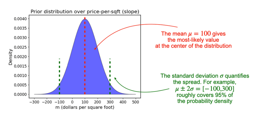
Visualizes how a large standard deviation broadens a normal prior around its mean. section 3.12