The Student’s t-distribution is a bell-shaped, symmetric distribution for estimating or testing a population mean from a small sample. It resembles the standard normal distribution, but its heavier tails leave more room for uncertainty when the sample’s variability is estimated rather than known. section 5.5 section 6.3
Think of estimating the average quality of an expensive product when only a few observations exist—perhaps 12 satellites, 5 bridges, or 10 candle batches. Getting more data may be impractical, so the t-distribution makes the resulting interval or test more cautious than a normal-distribution approach. section 5.5
Its main moving part is degrees of freedom:
- Use df = n − 1, where n is the sample size. section 5.5
- With fewer degrees of freedom, the tails are fatter, reflecting greater uncertainty. section 5.5
- As degrees of freedom approach 30, the t-distribution becomes very close to the normal distribution. section 5.5
Figure 5.8 The t-distribution with different degrees of freedom (DOF). Note that as the degrees of freedom approach 30, the distribution converges to a normal distribution.
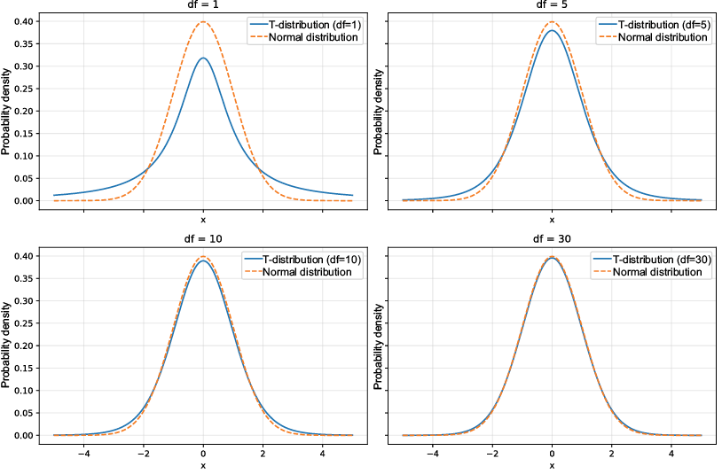
Compare the curves: low degrees of freedom produce visibly heavier tails; increasing degrees of freedom makes the t curve nearly overlap the normal curve. section 5.5
For a confidence interval, replace the normal critical value with a t critical value, then multiply it by the standard error. A 99% interval for a sample mean of 42.24, sample standard deviation 3.62, and n = 10 uses `stats.t.ppf(..., n-1)` to obtain that critical value. section 5.5
Testing a school-score claim
A college samples 21 students, observes a mean score of 110 and a sample standard deviation of 30, and tests whether its students score above a claimed mean of 100. Because the claim is directional, use a right-tailed one-sample t-test; compute the t statistic and obtain its p-value with `scipy.stats.t` using 20 degrees of freedom. section 6.12
The common small-sample guideline is to prefer t when n is 30 or fewer, assuming the population is normally distributed. For larger samples, normal and t approaches are very similar; many practitioners still use t because population variance is rarely known and consequences may be important. section 5.5 section 6.15