An array organizes numbers by position. A one-dimensional array is an indexed sequence; a matrix is a rectangular two-dimensional array with rows and columns; higher-dimensional arrays extend the same idea across more axes. This organization lets machine-learning systems carry structured inputs, intermediate layer values, and outputs rather than unrelated numbers. section 2.11.1 section 2.3
Array dimensions describe what each index selects. A vector is a one-dimensional tensor, a matrix is two-dimensional, an RGB image can be represented by color channel, height, and width, and a batch adds a leading batch dimension. Shape therefore records both the size and interpretation of each axis. section 2.12.5 section 2.11.1
Arrays commonly represent the following ML objects:
- A training dataset: rows are input instances and columns are feature elements. section 2.3
- An image: pixel values form a 2D array; color images combine R, G, and B arrays. section 2.11.1
- A neural-network value: inputs and outputs at each layer are tensors. section 2.11.1
- A minibatch of images: a four-dimensional array with batch, channel, height, and width axes. section 2.12.5
Indexing, slicing, and shape in PyTorch
A tensor holding eight two-feature training examples has shape 8 × 2. `X[0, 0]` selects its first element, `X[0, :]` selects its first row, and `X[:, 0]` selects its first column. Slices select ranges, such as the first three examples or one feature across several examples. PyTorch uses the same indexing ideas for image arrays, enabling channel selection and cropping. section 2.4
In convolution, the input is an array treated as a discrete signal. A small kernel array slides over it; at every position, corresponding elements are multiplied and summed into one output element. Kernel size, stride, and padding control which input positions contribute and how large the output array becomes. section 10.1 section 10.2
Figure 10.1 1D convolution with a local averaging kernel of size 3, stride 1, and valid padding on the input array of size 7
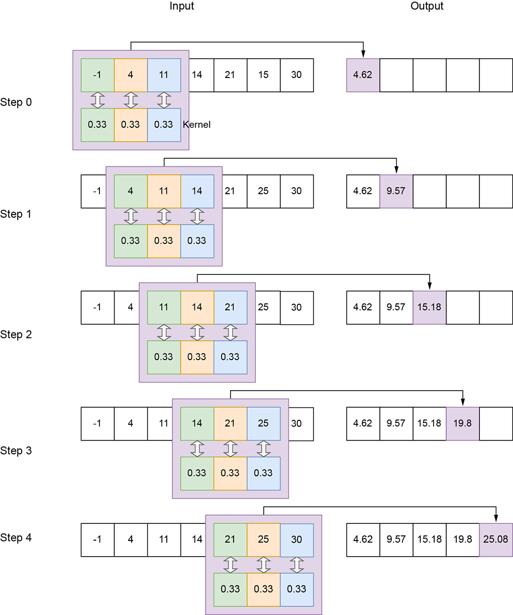
The sliding-kernel diagram makes the indexed, local nature of convolution visible: each kernel position consumes a window of the input array and emits one output value. section 10.1
For two-dimensional convolution, a single image array has height and width, but the PyTorch convolution interface expects a four-dimensional input: batch × channels × height × width. A grayscale image and its kernel can be expanded with singleton batch and channel axes before applying `Conv2d`. section 10.3.3