How deeply does Math and Architectures of Deep Learning cover variational autoencoder?

Derives ELBO-based training, explains stochastic encoding and reparameterization, and implements convolutional PyTorch components.

Variational autoencoder

As explained in Math and Architectures of Deep Learning

An autoencoder that models the latent space probabilistically and is trained with regularizing constraints.

A variational autoencoder (VAE) is an autoencoder that learns a probabilistic latent representation. Like an ordinary autoencoder, an encoder compresses an input and a decoder reconstructs it. Unlike an ordinary autoencoder, the encoder emits parameters of a latent distribution rather than one fixed latent vector, adding constraints that make the learned space compact and smooth. section 14.7 section 14.7.1 section 14.8

For a Gaussian latent family, the encoder produces a mean μ and covariance or variance parameters. Training samples z from that distribution, then the decoder maps z back to a reconstruction. At inference time, the mean μ can be used directly as the input’s latent representation. A narrow distribution keeps sampled points near its mean, while stochastic mapping lets the latent representation model uncertainty around an input. section 14.7.1 section 14.7.3

The objective balances reconstruction against regularization. Reconstruction loss asks the decoder to preserve the input; KL-divergence loss pushes the encoder’s learned latent distribution toward a chosen prior, commonly a zero-mean, unit-variance Gaussian. Without that constraint, reconstruction alone can place encoded training points far apart. With it, the model is encouraged to occupy less latent-space volume. section 14.6 section 14.7.8

This objective can also be derived through the evidence lower bound (ELBO). Minimizing divergence between the encoder’s approximate posterior q(z|x) and the unknown posterior is equivalent to maximizing the ELBO. Its entropy term favors a diffuse approximate distribution, supporting smoothness, while its expected joint-probability term connects latent representations and observed inputs. section 14.7.3 section 14.7.6

Sampling appears to block backpropagation because a random draw is not differentiable. The reparameterization trick separates randomness from learned parameters: draw ε from a fixed standard Gaussian, then compute z = μ + εσ. Gradients can therefore flow through μ and σ while randomness comes from ε. The same idea extends from one Gaussian variable to multivariate Gaussians. section 14.7.8

MNIST latent-space comparison

With a two-dimensional latent space on unlabeled MNIST digit images, both an autoencoder and a VAE can reconstruct test images well. The reconstruction-only autoencoder learns a sparse, widely spread latent space. The VAE adds KL regularization toward a standard Gaussian, yielding a visibly more compact latent space constrained within a unit ball. section 14.7.8

A PyTorch VAE training path is:

Encode an image with convolutional layers, then produce separate μ and log-variance vectors. section 14.7.8
Reparameterize by scaling standard-normal noise and adding μ, then decode z with transposed convolutions. section 14.7.8
Optimize binary cross-entropy reconstruction loss plus a weighted KL-divergence term. section 14.7.8

Figure 14.6 Two examples of mapping from a 2D input space to a 1D latent space. Both show regularized solid) vs. unregularized (dashed) latent space manifolds. Solid little circles depict training data points.

(a) Linear latent space

(b) Curved latent space

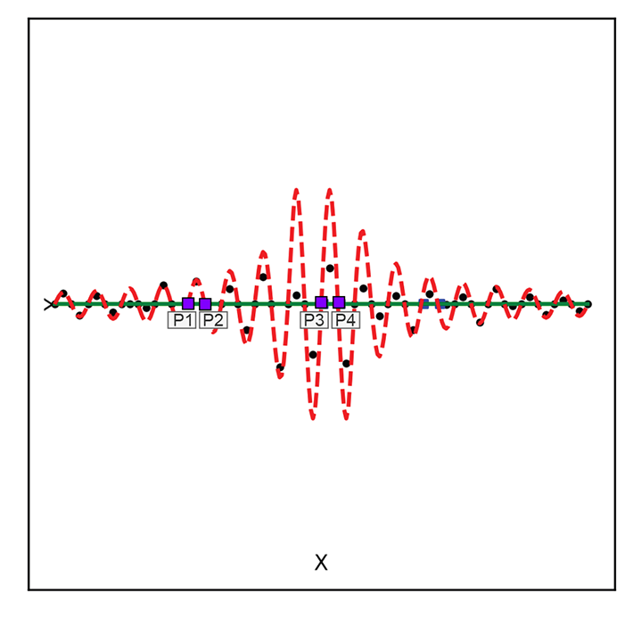
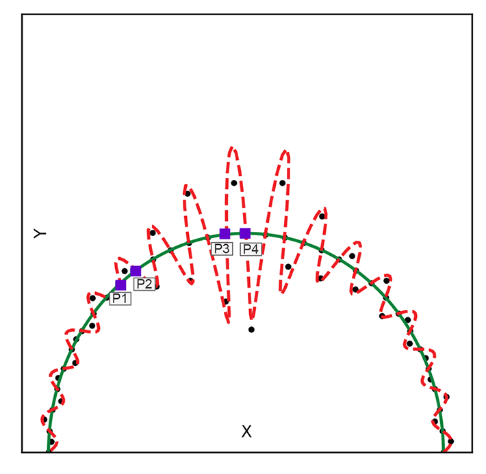
Compare regularized and unregularized mappings from a two-dimensional input space into one latent dimension; the regularized mappings keep training representations more compact. section 14.6

How Math and Architectures of Deep Learning covers it

Cover of Math and Architectures of Deep Learning

liveBook manning.com

Read Math and Architectures of Deep Learning on liveBook Get the book at manning.com

Also explained in

liveBook manning.com

Build a Text-to-Image Generator (from Scratch)A variational autoencoder is a generative neural model that encodes data into a lower-dimensional probabilistic latent representation and decodes that representation into reconstructed or generated data.
liveBook manning.com

Causal AIA variational autoencoder is a generative neural-network model that combines an encoder-defined approximating distribution with a decoder-defined generative distribution over observed data and latent variables.
liveBook manning.com

Learn Generative AI with PyTorchA generative model that learns an encoder-decoder latent-variable representation so it can reconstruct inputs and sample new outputs from latent space.
liveBook manning.com

Outlier Detection in PythonA variational autoencoder is a generative neural-network model that learns a probabilistic latent representation and reconstructs or generates observations from it.
liveBook manning.com

Deep Learning with Python, Third EditionA generative latent-variable model that learns an encoder-decoder structure and a probabilistic latent space for reconstructing and sampling data.
liveBook manning.com

Evolutionary Deep Learning: Genetic algorithms and neural networksA variational autoencoder is a neural network that encodes inputs as probability distributions, samples from those distributions, and decodes the samples to reconstruct or generate data.
liveBook manning.com

Generative AI in ActionA variational autoencoder is a generative neural model that encodes data into a probabilistic latent representation and decodes samples from that representation into reconstructed or newly generated data.
liveBook manning.com

Deep Learning with R, Third EditionA variational autoencoder is a probabilistic autoencoder whose encoder represents inputs as parameters of a latent probability distribution and whose decoder reconstructs or generates data from sampled latent points.
liveBook manning.com

Machine Learning Algorithms in DepthA variational autoencoder is a generative neural network that learns an approximate latent-variable posterior and reconstructs observations from sampled latent representations.
liveBook manning.com

Machine Learning for Tabular Data: XGBoost, Deep Learning, and AIA variational autoencoder is a neural network architecture that encodes data into a probabilistic latent space and decodes latent representations to reconstruct or generate data.
liveBook manning.com

Data Without LabelsA variational autoencoder is a neural-network generative model that learns a probabilistic latent representation and reconstructs data from sampled latent variables.
liveBook manning.com

Graph Neural Networks in ActionA variational autoencoder is a probabilistic autoencoder that learns a parameterized latent-variable distribution and decodes samples from it to reconstruct or generate data.

Compare how 13 books explain variational autoencoder →

Related concepts

encoderhas part · An encoder is a component that transforms input data into an encoded representation for subsequent processing, reconstruction, comparison, or transmission.
autoencoderkind of · An autoencoder is a neural network that encodes input data into an internal representation and decodes it to reconstruct the input or an approximation.
decodehas part · Decoding is the process of transforming an encoded or internal representation into an interpretable or target-form output.
generationkind of · Generation is the computational production of outputs from supplied inputs or context, often by applying a model to produce predictions or new content.
reconstruction lossuses · Reconstruction loss is a measure of the discrepancy between an input or observation and the output a model reconstructs from it or its representation.
image generationuses · Image generation is the computational creation of new images from learned models, input data, or specified conditions.

This explainer was generated by Manning's knowledge graph from the text of Math and Architectures of Deep Learning. The section links point to the parts of the book it draws on.