Intercept

As explained in Grokking Machine Learning

The value of a linear function when its input features are zero, corresponding to where the line crosses the y-axis.

Suppose a house-price model predicts 100 plus 50 for each room. The 50 tells you how much the predicted price rises with another room. What does the 100 do? It sets the starting height of the prediction line. section 3.2

The intercept, also called the y-intercept or bias, is where a line crosses the vertical axis. In y = mx + b, b is the intercept: when x is zero, mx is zero, so y equals b. For a model with several features, the bias is the prediction when all feature values are zero. The slope m is different: it controls how much the prediction changes as x increases. section 3.2

Figure 3.8 Some examples of slope and y-intercept. On the left, we see several lines with the same intercept and different slopes. Notice that the higher the slope, the steeper the line. On the right, we see several lines with the same slope and different y-intercepts. Notice that the higher the y-intercept, the higher the line is located.

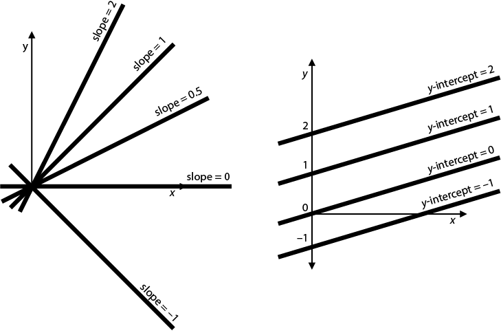
Compare the lines on the right: they have the same slope, but a higher intercept places the whole line higher. section 3.3

A house-price prediction

For Price = 100 + 50 × (number of rooms), the intercept is 100 and the slope is 50. A four-room house has a predicted price of 300. In a less tidy dataset, actual prices do not fall exactly on this line; the line gives predictions that can have small errors. section 3.2

Fitting a regression line means adjusting both its slope and intercept to bring it closer to the observed points. Changing the intercept moves the line up or down; changing the slope rotates it. In the square-trick update, the model first predicts a price, then adjusts its base price—the intercept—using the difference between the actual and predicted prices. section 3.3

You can also inspect a fitted intercept rather than calculate one by hand. In an area-only model for Hyderabad house prices, Turi Create reports an area coefficient of 9664.97 and an intercept of −6,105,981.01. The coefficient is the line’s slope; the intercept is its bias. Try fitting an area-only model and inspecting its coefficients, then compare the weights when you include other available features. section 3.5

How Grokking Machine Learning covers it

How deep it goes

Defines the axis crossing and zero-feature prediction, then shows how intercept updates move a single-feature regression line.

Examples

Uses a room-count price equation and an area-only Hyderabad housing model with a negative fitted intercept.

What it assumes

Introduces slope through rise over run and intercept through the axis crossing before using them as model parameters.

What you can do after

Apply it via Turi Create to inspect a fitted intercept alongside its feature coefficient.

How it connects

Connects linear regression, slope, weights, bias, features, and prediction error through line fitting.

liveBookmanning.com

Read Grokking Machine Learning on liveBook Get the book at manning.com

Also explained in

• 

  liveBookmanning.com
  Statistics Every Programmer NeedsAn intercept is the predicted value of a response variable when all predictors in a linear equation equal zero.
• 

  liveBookmanning.com
  Math and Architectures of Deep LearningA learned additive parameter that shifts model output independently of the inputs.
• 

  liveBookmanning.com
  Natural Language Processing in Action, Second EditionA bias is a constant input signal, conventionally equal to one, that allows a neuron to shift its activation independently of the other inputs.
• 

  liveBookmanning.com
  Data Without LabelsA bias term is a learnable additive neural-network parameter that shifts a unit's pre-activation independently of its weighted inputs.
• 

  liveBookmanning.com
  Grokking AI Algorithms, Second EditionA neural-network bias is a learned additive parameter that shifts a layer's computed output independently of its weighted inputs.
• 

  liveBookmanning.com
  Machine Learning Algorithms in DepthA bias parameter is a learned additive parameter that shifts a neural-network layer's preactivation values.

Compare how 7 books explain intercept →

Related concepts

• parameterkind of · A parameter is a value or variable that specifies or controls a characteristic, computation, or behavior of a function, model, operation, or request.
• thresholdequivalent to · A threshold is a boundary value against which a quantity is compared to determine whether a condition is met or an action or decision is triggered.
• classification scoreequivalent to · A classification score is a real-valued output representing a classifier’s support, confidence, or signed strength for a predicted class.
• line equationpart of · A line equation is an equation linear in its variables that represents a straight line in two dimensions or a linear relationship in higher dimensions.
• biasequivalent to · Bias is a systematic deviation or tendency in data, measurements, estimates, judgments, or outputs that skews them relative to a relevant target or impartial baseline.
• alphaequivalent to · Alpha is investment performance beyond a relevant benchmark or the return explained by specified systematic risk factors.

This explainer was generated by Manning's knowledge graph from the text of Grokking Machine Learning. The section links point to the parts of the book it draws on.