An intercept is the constant part of a linear model: the value predicted when every input is zero. In a housing rule, Price = 100 + 50 × rooms, the intercept is 100. It is the base price before adding anything for rooms; in machine learning, this constant is usually called the bias. section 3.2 section 3.4
For a one-feature line written as y = mx + b, b is the y-intercept. It marks where the line crosses the vertical axis, while m controls the line’s steepness. Changing the intercept moves the whole line up or down without changing its slope. section 3.11
Housing prediction
Suppose a fitted model has a price-per-room slope of 51.05 and an intercept of 99.10. For four rooms, it predicts 51.05 × 4 + 99.10 = 303.30. The intercept contributes the starting 99.10; the slope contributes the amount added for the rooms. section 3.18
With many features, there is still one intercept: ŷ = w1x1 + w2x2 + … + wnxn + b. Each weight changes the prediction according to one feature, while b remains the prediction’s constant starting value. Training adjusts both the weights and the intercept to move predictions closer to observed labels. section 3.19 section 3.6
An intercept also appears in classification. A perceptron adds its bias to the weighted feature score and predicts the positive class when that total is nonnegative. Equivalently, the bias is the negative of a threshold: a threshold of 3.5 becomes a bias of −3.5. section 5.4 section 5.5
Empty-input score
For a sentiment classifier, an empty sentence has no word weights to add, so its score is exactly the bias. A positive bias places it in the positive class; a negative bias places it in the negative class. section 5.10
Figure 3.8 Some examples of slope and y-intercept. On the left, we see several lines with the same intercept and different slopes. Notice that the higher the slope, the steeper the line. On the right, we see several lines with the same slope and different y-intercepts. Notice that the higher the y-intercept, the higher the line is located.
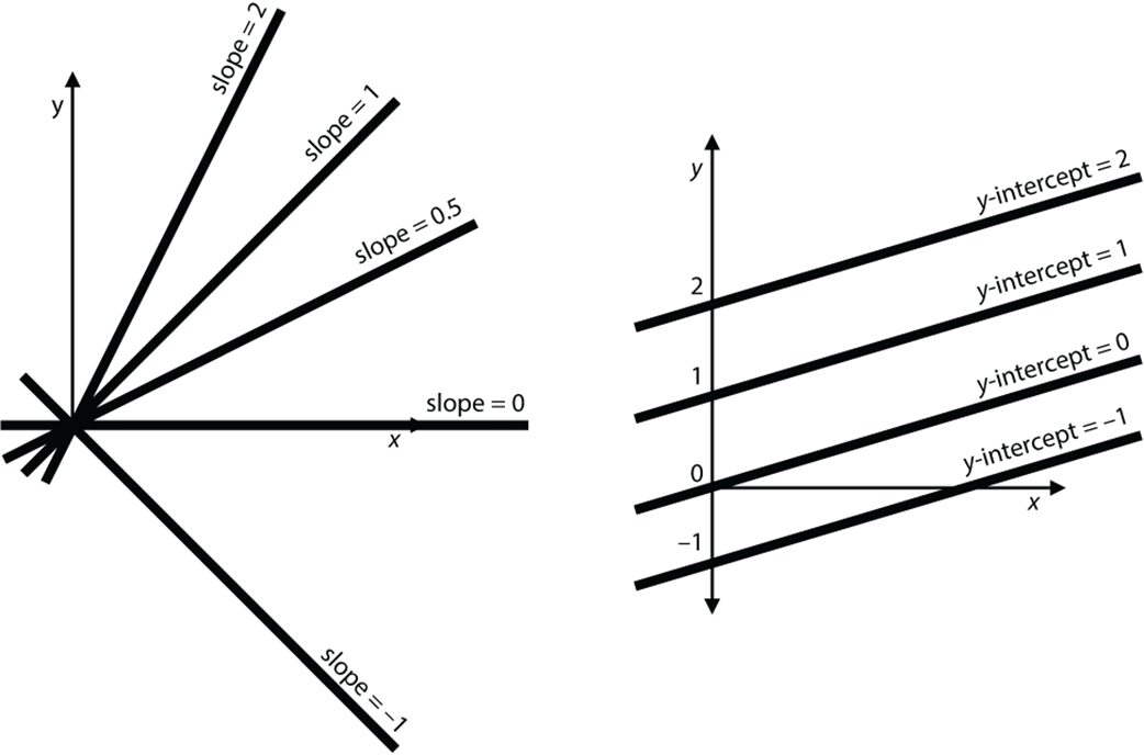
Compare lines with matching slopes or matching intercepts to see that the intercept changes vertical location, not steepness. section 3.11
In scikit-learn linear regression, the learned intercept is available separately from the feature coefficients. For an area-and-price model, the coefficient is the slope and the intercept is the bias. section 3.27