The Central Limit Theorem (CLT) is the reason a messy population can still produce a tidy bell curve. When many sufficiently large random samples are taken and each sample is reduced to its mean, the distribution of those means approaches a normal distribution—even when the original data are skewed. This links samples to population inference without claiming that any one sample perfectly represents the population. section 4.9 section 4.12
Think of each sample mean as one attempt at estimating a population average. The sampling distribution is the collection of those attempts. Its center equals the population mean, while its spread is the population standard deviation divided by the square root of the sample size: σₓ̄ = σ/√n. Bigger samples therefore make sample means less variable and the bell curve narrower. section 5.1 section 5.1
From lopsided tornado widths to bell-shaped means
Recorded tornado widths are heavily right-skewed, not bell-shaped. Repeatedly draw random samples of 45 widths, calculate each mean, and plot 1,000 means. The resulting histogram appears normal, illustrating that the CLT concerns a distribution of sample means rather than the shape of individual tornado widths. section 4.9 section 4.9
Use the CLT by keeping these distinctions straight:
- A sample mean is the average within one sample; the mean of sample means is the average across many samples. section 5.1
- A normally distributed population gives normally distributed sample means; a nonnormal population can also do so when samples are large enough. section 5.1
- For sample proportions, check the rules of thumb n·p ≥ 5 and n·(1−p) ≥ 5 before using a normal approximation. section 5.7
- For proportions, use standard error rather than the population standard deviation when constructing the bell curve. section 5.7
The theorem turns sample averages into probability questions. For adults with population mean body temperature 98.2°F and standard deviation 0.73°F, a sample of 31 has a sampling-distribution mean of 98.2 and standard deviation 0.73/√31. A normal CDF gives P(sample mean < 98°F) = 0.0636. The result describes the likelihood of a sample average, not the likelihood that an individual person is below 98°F. section 5.1 section 5.1
Figure 5.2 Increasing the sample size n narrows the bell curve and decreases uncertainty in the sample means.
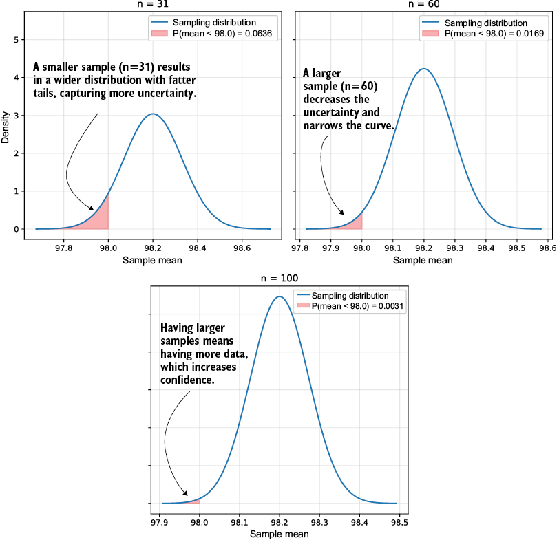
Compare sample sizes 31, 60, and 100: increasing n narrows the sampling distribution and reduces uncertainty around the sample mean. section 5.1
This normal approximation supports confidence intervals: instead of reporting one sample estimate as certainty, report a range of plausible population values at a stated confidence level. Sampling quality still matters. A survey drawn from venues with a particular demographic can bias a proportion estimate, even when the normal-approximation conditions are met. section 5.0 section 5.7


