A dark cloud can change your estimate of today’s chance of rain. Conditional probability describes a chance after taking specified information into account. If X is rain and D is the observed cloud, Pr(X | D) means the probability of rain given that observation. The vertical bar means “given.” Pr(X), without the condition, represents the chance before that observation. section 1.5 section 2.2
In Bayesian reasoning, the probability of a hypothesis given observed data is its posterior probability. Bayes’ theorem connects that posterior to two other quantities: the prior probability of the hypothesis and the likelihood of seeing the data if the hypothesis were true. To compare hypotheses, multiply each prior by its likelihood, then divide each result by the sum of those products. The resulting posterior probabilities sum to 1. section 2.2
A positive test for a rare disease
Suppose a disease affects about 1 in 150 people. A test is positive for 98% of people with the disease, but also for 5% of people without it. The first figure is Pr(positive test | disease); the question you care about is Pr(disease | positive test). Combining the test results with the disease’s low prior probability gives a probability of only about 12% after a positive result. A positive test therefore does not, by itself, make the disease nearly certain. section 2.5
The direction of the condition matters. A small probability of observing evidence if someone is innocent, Pr(evidence | innocence), is not automatically a small probability of innocence given the evidence, Pr(innocence | evidence). Assessing the latter also requires prior probabilities and the likelihood of the evidence under alternative explanations. section 11.7
Conditional probability also describes prediction from context. For a next-word prediction, a starting phrase helps determine which continuations are more likely. This is an application of conditioning, though language models described this way are not necessarily fully Bayesian models. section 1.7
Figure 2.1 Bayes’ theorem and the interpretation of its components.
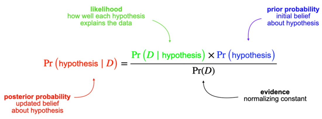
The diagram links the prior, likelihood, and posterior in Bayes’ theorem, making clear which probability is conditioned on the observed data. section 2.2