A small image dataset can let a classifier memorize its training pictures instead of learning to recognize new ones. Data augmentation creates believable variations of existing training images with random transformations. The aim is to show the model different versions of a picture as training proceeds, helping it generalize. section 8.2.5 section 8.2.4
Augment cat and dog pictures
For a cat–dog classifier, apply random horizontal flips, rotations, and zooms to training images while leaving their cat or dog labels unchanged. In R/Keras, put these layers in a function that returns the transformed images with their original targets, then map it over the training Dataset. section 8.2.5
Listing 8.18 Defining a data augmentation stage
data_augmentation_layers <- list(  #1
  layer_random_flip(, "horizontal"),
  layer_random_rotation(, 0.1),
  layer_random_zoom(, 0.2)
)

data_augmentation <- function(images, targets) {  #2
  for (layer in data_augmentation_layers)
    images <- layer(images)
  list(images, targets)
}

augmented_train_dataset <- train_dataset |>
  dataset_map(data_augmentation, num_parallel_calls = 8) |>  #3
  dataset_prefetch() #4
The complete R/Keras augmentation stage maps three random image transformations over training batches, retains the targets, and prefetches batches. section 8.2.5
Figure 8.10 Generating variations of a very good cat via random data augmentation
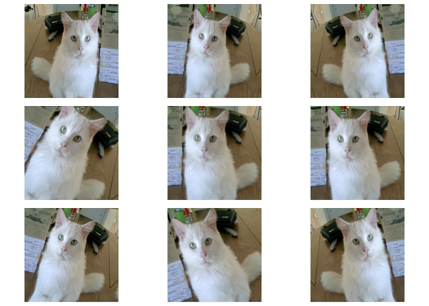
Repeated transformations of one cat image show the variety the model can encounter without collecting another labeled picture. section 8.2.5
The augmentation layers can run inside the model, before rescaling, or outside it in the data pipeline. The first option runs on the GPU; the mapped pipeline runs on the CPU, typically across multiple cores. The pipeline approach is generally preferred here, though either may be faster in a particular setup. Augment training data, but keep the validation dataset unchanged when fitting the model. section 8.2.5
Check the result, not just the training curve
A small convnet trained on 2,000 cat–dog images reached 79.3% test accuracy before augmentation. A later model trained on augmented images reached 82.9%. That later model also added dropout, so the difference is not an isolated measure of augmentation’s effect. section 8.2.4 section 8.2.5
Augmentation also affects how pretrained features are used. Computing and storing each image’s features once is fast, but cannot produce new transformed inputs on later passes. Running images through a frozen pretrained convolutional base during training permits augmentation, at greater computational cost. section 8.3.1








