A feature map keeps track of what a convolutional network detects and where it detects it. It has height, width, and channels. Each channel is a two-dimensional response map: its values indicate how strongly one learned filter responds at different image locations. An RGB input has three color channels; after a convolution, channels represent learned filters instead. section 8.1.1
Follow the shapes in a digit classifier
In R/Keras, start with `keras_input(shape = c(28, 28, 1))`, then apply `layer_conv_2d(filters = 64, kernel_size = 3, activation = "relu")` and `layer_max_pooling_2d(pool_size = 2)`. The 28 × 28 grayscale input becomes a 26 × 26 × 64 feature map: 64 response maps, each covering 26 × 26 locations. Pooling then changes its shape to 13 × 13 × 64. Later convolutions can combine simple local patterns, such as edges, into larger patterns. section 8.1 section 8.1.1
Figure 8.3 The concept of a response map: a 2D map of the presence of a pattern at different locations in an input
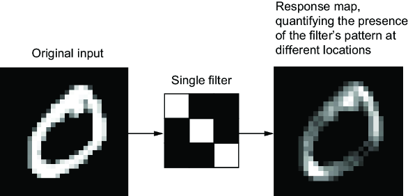
The diagram makes the key distinction visible: one channel is a two-dimensional response map; multiple channels together form the feature map. section 8.1.1
Convolution applies the same learned transformation to patches throughout an input feature map. That lets a filter respond to a pattern at different positions without learning the pattern separately at each position. The number of output channels is chosen by the layer’s filter count; height and width depend on how patches are taken. section 8.1.1
Feature maps commonly become smaller across successive layers while gaining channels. Max pooling typically takes the maximum in each channel over a 2 × 2 window with stride 2. Shrinking the maps helps later features draw on larger portions of the original image. Without downsampling, a digit classifier’s final maps can remain 22 × 22, leaving much spatial information to discard at global average pooling. section 8.1.2 section 8.2.3
What happens next depends on the task. For image classification, global average pooling turns each channel into one value for a dense classifier. For segmentation, locations must remain useful for per-pixel predictions: strided convolutions downsample the maps, and transposed convolutions restore spatial dimensions. Max pooling is less suitable there because it loses which position within a window supplied its maximum. section 8.1 section 11.3.2
Feature maps can also be reused or inspected. A pretrained convolutional backbone supplies spatial features for a new classifier; earlier layers tend to capture generic edges, colors, and textures, while later ones capture more abstract patterns. To inspect a model, collect its convolution and pooling outputs for an image and plot each channel separately as a two-dimensional image. In a cat-image example, one first-layer channel appears to respond to diagonal edges, though learned channels can vary. section 8.3.1 section 10.1
Listing 10.5 Visualizing the sixth channel
plot_activations <- function(x, ...) {
  withr::local_par(list(mar = c(0,0,0,0)))

  x <- drop(as.array(x))
  if (sum(x) == 0)
    return(plot(as.raster("gray")))

  rotate <- function(x) t(apply(x, 2, rev))
  graphics::image(
    rotate(x), asp = 1, axes = FALSE, useRaster = TRUE,
    col = viridis::viridis(256), ...
  )
}plot_activations(first_layer_activation[, , , 6])
The R plotting example selects one channel from a first-layer activation, showing how to inspect a feature map rather than treating all its channels as one image. section 10.1







