Feature map

As explained in Sutskever's List

A spatial array of responses produced by applying a convolutional filter to an input.

A feature map is a spatial array of responses produced when a convolutional filter compares its learned pattern with image regions. Applying the same filter across the image shows where that pattern appears; multiple filters produce multiple maps. section 2.5.1

From edges to object parts

In AlexNet, 96 filters in the first convolutional layer produce 96 feature maps. Early maps can respond to edges; deeper layers combine patterns into contours and recognizable parts, such as ears or whiskers. section 2.5.1

Figure 2.3 The AlexNet architecture (cropped in the original paper). The numbers indicate spatial dimensions and channel depth at each stage. The input image (224 × 224 × 3 RGB) passes through a series of convolutional and pooling layers that progressively reduce spatial resolution (224→55→27→13) while increasing channel depth. Early downsampling is driven by the first convolutional layer (11 × 11 filters with a stride of 4), followed by max pooling layers (3 × 3 windows with a stride of 2) that further reduce spatial dimensions. The stride determines how far a filter moves across the input at each step, controlling how densely the image is sampled and how quickly spatial resolution is reduced. Filter sizes (11, 5, 3) are depicted as cubes and define the local receptive field of each convolution. The two horizontal streams reflect the model’s original two-GPU training setup, where feature maps were split across devices (e.g., 48 + 48 = 96 channels). The fully connected layers (4096 neurons, implemented as 2048 + 2048 across GPUs) feed into a 1000-way output for ImageNet classification. Used with permission granted by the lead author (Alex Krizhevsky).

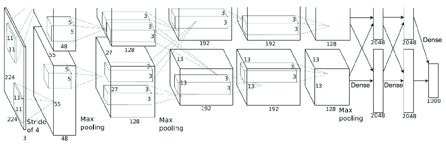
The architecture diagram shows feature-map channels across AlexNet’s layers and how pooling reduces their spatial dimensions. section 2.5.1

How Sutskever's List covers it

How deep it goes

Defines feature maps through filter responses and traces their progression from edges to object parts.

Examples

Illustrates 96 first-layer AlexNet maps and the progression from edge responses to contours and object parts.

What you can do after

Understand how convolutional filters produce spatial responses that deeper layers can combine into more abstract visual patterns.

How it connects

Links feature maps to convolutional layers, filters, max pooling, and translation invariance.

liveBookmanning.com

Read Sutskever's List on liveBook Get the book at manning.com

Also explained in

• 

  liveBookmanning.com
  Deep Learning with R, Third EditionA feature map is a spatial array of activations indicating the presence or strength of a learned visual pattern at different image locations.
• 

  liveBookmanning.com
  Grokking Machine LearningA mapping that sends data points from an original input space into another feature space, usually of higher dimension.
• 

  liveBookmanning.com
  Grokking AI Algorithms, Second EditionA feature map is a spatially organized array of activation values representing learned features at different locations in an input or intermediate image representation.
• 

  liveBookmanning.com
  Math and Architectures of Deep LearningA spatial array of activation values produced by applying a convolution or pooling operation over an input image or prior layer output.
• 

  liveBookmanning.com
  Deep Learning with Python, Third EditionA spatial grid of activations produced by a convolutional or pooling layer, where each channel encodes the presence of a learned feature over locations.
• 

  liveBookmanning.com
  Learn Generative AI with PyTorchAn intermediate activation map in a neural network whose spatial resolution can be increased or preserved by convolutional operations.
• 

  liveBookmanning.com
  Machine Learning Algorithms in DepthA feature map is a function that represents input objects as vectors in a feature space, possibly an infinite-dimensional one.

Compare how 8 books explain feature map →

Related concepts

• convolutional layerproduced by · A convolutional layer is a neural-network layer that applies shared learned filters to local regions of structured input to produce feature representations.
• kernel functionproduced by · A kernel function is a mathematical function that measures similarity between pairs of inputs, often representing an inner product in an implicit feature space.
• convolution kernelproduced by · A convolution kernel is a small array or tensor of weights applied across local input regions to compute weighted responses and detect or transform patterns.
• Region Proposal Networkused by · A Region Proposal Network is a neural-network module that generates candidate object regions from image features for a two-stage detector.
• channelhas part · A channel is an independent component or dimension of image or tensor data carrying a distinct color, feature, activation, or value stream.
• max poolingused by · Max pooling is an aggregation operation that replaces each local or grouped region with its maximum value, often to downsample a representation.

This explainer was generated by Manning's knowledge graph from the text of Sutskever's List. The section links point to the parts of the book it draws on.