Feature map

As explained in Math and Architectures of Deep Learning

A spatial array of activation values produced by applying a convolution or pooling operation over an input image or prior layer output.

A feature map is a spatial grid of learned activations produced when a convolutional layer scans an image or an earlier layer’s output. Each grid value summarizes information from a local input region, so the grid preserves both what was detected and approximately where it was detected. Stacking convolutional layers turns early maps for simple patterns, such as lines and edges, into later maps for more abstract structures. section 10.7 section 11.2

Feature maps are not merely intermediate arrays: they are the representation a convolutional network passes forward. A layer can produce multiple maps, with each map corresponding to a learned filter. In LeNet, a first convolution produces six 28 × 28 feature maps; later convolutions produce 16 maps of size 10 × 10 and then 120 maps of size 1 × 1, which are flattened into a vector for fully connected layers. section 11.1

Spatial resolution and receptive fields determine what a feature map represents:

• A grid point is a digest of the input patch in its receptive field. One 5 × 5 convolution and two successive 3 × 3 convolutions can give an output point the same 5 × 5 receptive field. section 11.2
• Deeper stacks can reach the same input area with fewer filter parameters: two 3 × 3 filters use 18 parameters versus 25 for one 5 × 5 filter in the single-channel example. section 11.2
• Pooling downsamples a feature map by summarizing local patches with a maximum or average. This reduces resolution and makes feature locations less sensitive to small shifts and distortions. section 10.7
• Kernel size and stride control output size. A 2 × 2 pooling kernel with stride 2 halves each spatial dimension; a 3 × 3 kernel with stride 3 reduces it to one-third. section 10.7

Pooling a feature map

Given a 4 × 4 activation grid, max pooling with a 2 × 2 kernel and stride 2 divides it into four local patches and emits one maximum from each patch. The result is a 2 × 2 feature map: lower resolution, but still retaining the strongest activation in every patch. In PyTorch, torch.nn.MaxPool2d(kernel_size=2, stride=2) performs this operation; AvgPool2d uses each patch average instead. section 10.7

Figure 10.19 Max pooling using a 2 × 2 kernel with stride 2. The resulting output feature map is half the size of the input feature map. Each value of the output feature map is a max of the corresponding local patch in the input feature map.

Inspect the 2 × 2 max-pooling layout to see how each output feature-map value summarizes one local input patch and halves spatial resolution. section 10.7

For image classification, repeated convolution, activation, and pooling transform image-sized maps into compact representations for prediction. Pooling after LeNet’s first two convolutional layers halves map resolution and reduces sensitivity to input shifts and distortions, while tanh activations add the nonlinearity needed for the network to model nonlinear combinations of inputs. section 11.1

For object detection, a convolutional backbone computes a feature map once for the whole image. A region of interest can then be mapped onto that grid using the backbone’s subsampling factor. With a factor of 16, a 256 × 256 image region corresponds to a 16 × 16 region on the convolutional feature map. RoI pooling extracts fixed-size features from such regions, allowing many RoIs to share one backbone forward pass before classification and bounding-box regression. section 11.4 section 11.4.3

Figure 11.18 A conv feature map with two regions of interest of different sizes. RoI pooling extracts a fixed-sized output feature map (2 × 2 in this image) from each of the RoIs in a single pass via max pooling. This enables us to extract fixed-sized representative feature vectors for each RoI, which are then fed into further classifier and regressor layers for classification and localization.

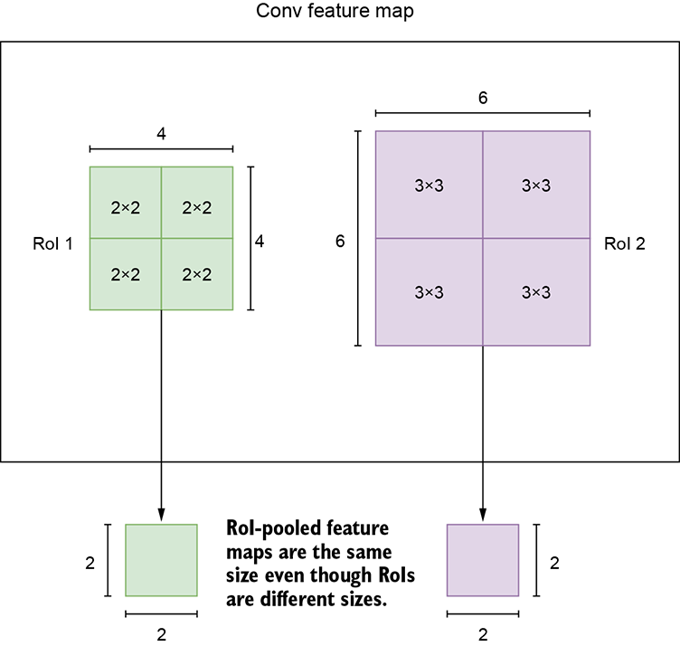
Compare differently sized regions of interest on one convolutional feature map and see how RoI pooling produces fixed-sized outputs for classification and localization. section 11.4.3

How Math and Architectures of Deep Learning covers it

How deep it goes

Explains spatial summaries, pooling resolution changes, receptive fields, and RoI extraction without deriving convolution arithmetic.

Examples

Uses LeNet map dimensions, 2 × 2 max and average pooling, stacked 3 × 3 convolutions, and RoI pooling.

What it assumes

Introduces feature-map roles through images and convolution layers while assuming familiarity with neural-network layers and spatial kernels.

What you can do after

Evaluate/understand how convolutional representations retain spatial information while supporting classification and region feature extraction.

How it connects

Connects convolution, pooling, receptive fields, activation functions, LeNet, Faster R-CNN, and RoI pooling.

liveBookmanning.com

Read Math and Architectures of Deep Learning on liveBook Get the book at manning.com

Also explained in

• 

  liveBookmanning.com
  Deep Learning with R, Third EditionA feature map is a spatial array of activations indicating the presence or strength of a learned visual pattern at different image locations.
• 

  liveBookmanning.com
  Grokking Machine LearningA mapping that sends data points from an original input space into another feature space, usually of higher dimension.
• 

  liveBookmanning.com
  Grokking AI Algorithms, Second EditionA feature map is a spatially organized array of activation values representing learned features at different locations in an input or intermediate image representation.
• 

  liveBookmanning.com
  Deep Learning with Python, Third EditionA spatial grid of activations produced by a convolutional or pooling layer, where each channel encodes the presence of a learned feature over locations.
• 

  liveBookmanning.com
  Sutskever's ListA spatial array of responses produced by applying a convolutional filter to an input.
• 

  liveBookmanning.com
  Learn Generative AI with PyTorchAn intermediate activation map in a neural network whose spatial resolution can be increased or preserved by convolutional operations.
• 

  liveBookmanning.com
  Machine Learning Algorithms in DepthA feature map is a function that represents input objects as vectors in a feature space, possibly an infinite-dimensional one.

Compare how 8 books explain feature map →

Related concepts

• convolutional layerproduced by · A convolutional layer is a neural-network layer that applies shared learned filters to local regions of structured input to produce feature representations.
• kernel functionproduced by · A kernel function is a mathematical function that measures similarity between pairs of inputs, often representing an inner product in an implicit feature space.
• convolution kernelproduced by · A convolution kernel is a small array or tensor of weights applied across local input regions to compute weighted responses and detect or transform patterns.
• Region Proposal Networkused by · A Region Proposal Network is a neural-network module that generates candidate object regions from image features for a two-stage detector.
• channelhas part · A channel is an independent component or dimension of image or tensor data carrying a distinct color, feature, activation, or value stream.
• max poolingused by · Max pooling is an aggregation operation that replaces each local or grouped region with its maximum value, often to downsample a representation.

This explainer was generated by Manning's knowledge graph from the text of Math and Architectures of Deep Learning. The section links point to the parts of the book it draws on.