Convolution kernel

As explained in Deep Learning with Python, Third Edition

The learned weight tensor used by a convolution to transform local input patches.

A convolution kernel is the learned weight tensor behind a filter. It transforms a small patch of an input feature map, then applies that same transformation as the window moves across the image. Instead of looking for a pattern only in one place, the filter produces a response at many locations. section 8.1.1

A filter over an MNIST digit

A Conv2D(64, (3, 3)) layer uses 3 × 3 patches and computes 64 filters. For a (28, 28, 1) MNIST input, the illustrated output is (26, 26, 64). Each output channel is a 26 × 26 response map: it shows where one filter responded. The input’s single channel represents grayscale; the output’s 64 channels represent learned filters, not colors. section 8.1.1

Figure 8.4 How convolution works

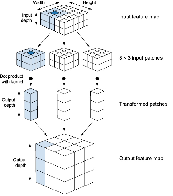
Follow one window across the input to see why a single kernel yields responses at multiple locations. section 8.1.1

Keep two layer choices separate:

• Window size determines the size of each local patch; 3 × 3 and 5 × 5 are typical choices. section 8.1.1
• Output depth determines how many filters—and therefore how many response maps—the layer computes. In Keras, these are the arguments in Conv2D(output_depth, (window_height, window_width)). section 8.1.1

What a filter responds to changes through a ConvNet. Earlier filters may detect edges or basic textures; later ones may respond to more abstract concepts. A response map shows *where* a filter responds in an image. To inspect *what pattern* prompts that response, start with a blank image and adjust its pixels to maximize the chosen filter’s activation. section 10.2 section 10.5

Inspecting a trained filter

With a KerasHub Xception model trained on ImageNet, select a Conv2D or SeparableConv2D layer, then make a feature extractor from its output: keras.Model(inputs=model.input, outputs=layer.output). After model-specific image preprocessing, measure one output channel’s mean activation and optimize the input image to increase it. The resulting image illustrates the pattern that filter responds to; it is not the filter’s weight tensor. section 10.2

How Deep Learning with Python, Third Edition covers it

How deep it goes

Defines patch size, filter count, and response maps, then works through filter visualization without deriving kernel-weight calculations.

Examples

Uses a 3 × 3 MNIST convolution and filter-activation optimization on a pretrained Xception model.

What it assumes

Assumes basic familiarity with images and neural-network layers while explaining image channels, feature maps, and filter responses through MNIST.

What you can do after

Diagnose/debug with it by inspecting a filter’s response map or optimizing an input image to reveal its preferred pattern.

How it connects

Connects convolution kernels to feature maps, output channels, receptive visual patterns, and activation visualization.

liveBookmanning.com

Read Deep Learning with Python, Third Edition on liveBook Get the book at manning.com

Also explained in

• 

  liveBookmanning.com
  Natural Language Processing in Action, Second EditionA convolutional kernel is a parameter matrix or tensor whose sliding weighted operation detects a local pattern in an input sequence.
• 

  liveBookmanning.com
  Math and Architectures of Deep LearningA learned kernel applied in a convolution layer to detect local spatial patterns in images.
• 

  liveBookmanning.com
  Inside Deep Learning: Math, Algorithms, ModelsA learned array of weights applied over local input regions to compute convolution outputs.
• 

  liveBookmanning.com
  Deep Learning with PyTorch, Second EditionA small learned filter window applied over local regions of an input to compute weighted sums.
• 

  liveBookmanning.com
  Grokking AI Algorithms, Second EditionA convolutional filter is a small learned grid of weights that detects a particular local pattern in image data.
• 

  liveBookmanning.com
  Deep Learning with R, Third EditionA convolution kernel is a learned weight matrix that transforms each extracted input patch into an output feature vector.
• 

  liveBookmanning.com
  Graph Neural Networks in ActionA learnable weighted operation that transforms input data to emphasize particular patterns or features.
• 

  liveBookmanning.com
  Learn Generative AI with PyTorchA learned convolutional kernel whose weights slide across local input regions to produce feature responses.
• 

  liveBookmanning.com
  Sutskever's ListA convolutional kernel is a grid of learned weights applied across local regions of an input to produce spatial responses.
• 

  liveBookmanning.com
  Evolutionary Deep Learning: Genetic algorithms and neural networksA convolutional filter is a learned array of weights that is slid across local input regions to produce feature responses.

Compare how 11 books explain convolution kernel →

Related concepts

• convolutional neural networkused by · A convolutional neural network is a neural-network architecture that applies learned convolutional operations to extract patterns from structured data.
• convolutional layerused by · A convolutional layer is a neural-network layer that applies shared learned filters to local regions of structured input to produce feature representations.
• feature mapproduces · A feature map is a spatially organized array of neural-network activations representing the presence or strength of learned features at different locations.
• image processinguses · Image processing is the computational manipulation and analysis of digital image data to transform images or extract information.

This explainer was generated by Manning's knowledge graph from the text of Deep Learning with Python, Third Edition. The section links point to the parts of the book it draws on.