Convolution kernel

As explained in Math and Architectures of Deep Learning

A learned kernel applied in a convolution layer to detect local spatial patterns in images.

A convolution kernel is a small array of weights that slides across an input and emits one output value at each position. At every slide stop, corresponding input values and kernel weights are multiplied and summed: the result is a weighted local sum. Because each output depends only on a nearby patch, kernels capture local patterns rather than connecting every input to every output. section 10.1 section 10.8

Kernel weights determine what pattern receives a strong response. Equal, normalized weights compute a local average and smooth short-term variation. Positive and negative weights can suppress uniform regions while responding strongly where values change abruptly, making edges visible. In trained convolution layers, kernel weights are normally learned rather than manually chosen. section 10.1.1 section 10.1.2 section 10.1.4

A kernel is defined by its shape and how it is applied:

• In one dimension, a short weight vector slides along an array like a ruler over a rope; each position produces one output element. section 10.1
• In two dimensions, a tile-shaped kernel computes weighted sums over neighboring image pixels, supporting smoothing and horizontal or vertical edge detection. section 10.3.1 section 10.3.2
• In three dimensions, a brick-shaped kernel spans time, height, and width in a video volume, so its weights can compare successive frames and respond to motion. section 10.4 section 10.4.1
• Kernel size, stride, and padding determine which local regions are visited and affect output size; zero padding supplies zeros outside the input boundary. section 10.2 section 10.8

From local averaging to edge detection

For a 1D input, a three-weight uniform kernel produces the moving average of each neighboring triple, reducing noise and revealing the broader trend. Replacing it with an antisymmetric two-weight kernel makes the output spike where adjacent values jump. The same contrast applies to images: a uniform 2D kernel denoises a noisy text image, while an edge kernel emphasizes boundaries and suppresses flat areas. section 10.1.1 section 10.1.2 section 10.3.1 section 10.3.2

A convolution can also be expressed as matrix-vector multiplication: repeated placements of the same kernel create a structured weight matrix. This links convolution to linear layers and allows forward propagation and backpropagation to use the same underlying training principles, while preserving local connectivity. section 10.1.3

In PyTorch, Conv1d, Conv2d, and Conv3d accept convolution parameters and hold weight tensors. Inputs include batch and channel dimensions; for 2D inputs the expected layout is N × C × H × W. Explicitly assigning custom weights is useful for inspecting the operation, whereas practical networks usually learn the weights during training. section 10.1.4 section 10.3.3 section 10.4.2

Figure 10.1 1D convolution with a local averaging kernel of size 3, stride 1, and valid padding on the input array of size 7

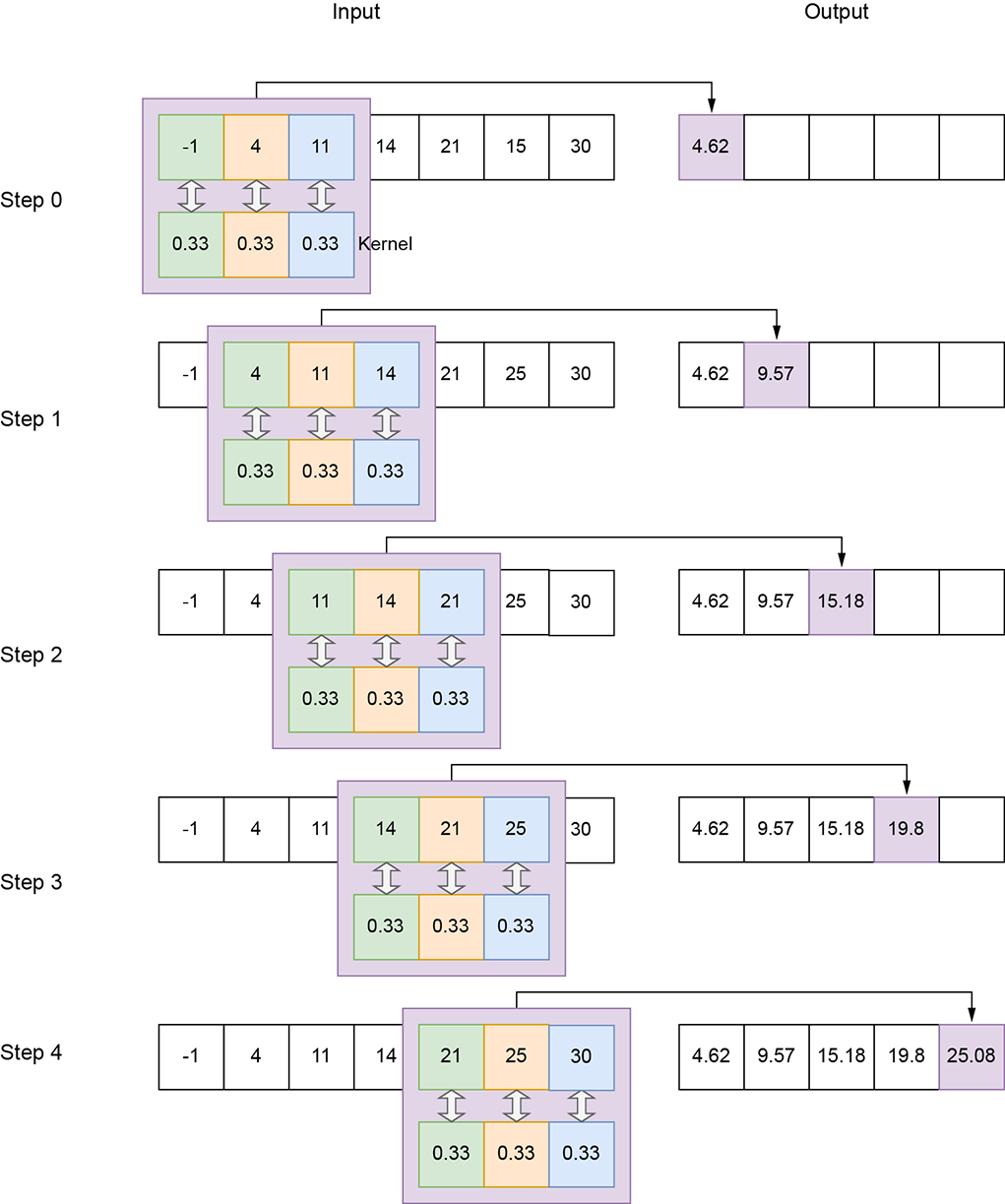
Follow the shaded three-weight kernel across a 1D input to see how one local weighted sum is emitted at every slide stop. section 10.1

How Math and Architectures of Deep Learning covers it

How deep it goes

Derives sliding weighted sums and output sizing, then relates convolution to matrix multiplication and backpropagation.

Examples

Uses moving-average curves, edge-detection signals, noisy text images, image boundaries, and a moving-ball video.

What it assumes

Builds convolution intuition from discrete arrays before extending weighted local sums to images and video.

What you can do after

Apply it via PyTorch Conv1d, Conv2d, and Conv3d by setting kernel weights and tensor shapes for demonstrations.

How it connects

Connects convolution kernels to stride, padding, linear layers, backpropagation, receptive fields, and feature maps.

liveBookmanning.com

Read Math and Architectures of Deep Learning on liveBook Get the book at manning.com

Also explained in

• 

  liveBookmanning.com
  Natural Language Processing in Action, Second EditionA convolutional kernel is a parameter matrix or tensor whose sliding weighted operation detects a local pattern in an input sequence.
• 

  liveBookmanning.com
  Inside Deep Learning: Math, Algorithms, ModelsA learned array of weights applied over local input regions to compute convolution outputs.
• 

  liveBookmanning.com
  Deep Learning with PyTorch, Second EditionA small learned filter window applied over local regions of an input to compute weighted sums.
• 

  liveBookmanning.com
  Grokking AI Algorithms, Second EditionA convolutional filter is a small learned grid of weights that detects a particular local pattern in image data.
• 

  liveBookmanning.com
  Deep Learning with Python, Third EditionThe learned weight tensor used by a convolution to transform local input patches.
• 

  liveBookmanning.com
  Deep Learning with R, Third EditionA convolution kernel is a learned weight matrix that transforms each extracted input patch into an output feature vector.
• 

  liveBookmanning.com
  Graph Neural Networks in ActionA learnable weighted operation that transforms input data to emphasize particular patterns or features.
• 

  liveBookmanning.com
  Learn Generative AI with PyTorchA learned convolutional kernel whose weights slide across local input regions to produce feature responses.
• 

  liveBookmanning.com
  Sutskever's ListA convolutional kernel is a grid of learned weights applied across local regions of an input to produce spatial responses.
• 

  liveBookmanning.com
  Evolutionary Deep Learning: Genetic algorithms and neural networksA convolutional filter is a learned array of weights that is slid across local input regions to produce feature responses.

Compare how 11 books explain convolution kernel →

Related concepts

• convolutional neural networkused by · A convolutional neural network is a neural-network architecture that applies learned convolutional operations to extract patterns from structured data.
• convolutional layerused by · A convolutional layer is a neural-network layer that applies shared learned filters to local regions of structured input to produce feature representations.
• feature mapproduces · A feature map is a spatially organized array of neural-network activations representing the presence or strength of learned features at different locations.
• image processinguses · Image processing is the computational manipulation and analysis of digital image data to transform images or extract information.

This explainer was generated by Manning's knowledge graph from the text of Math and Architectures of Deep Learning. The section links point to the parts of the book it draws on.