A gradient indicates how an objective changes as model parameters change. In optimization, it guides the correction to model weights that reduces error at the current step. Gradient descent starts from an initial set of weights, computes error and its gradient, then repeats weight updates toward a lower-error solution. section 4.3.5 section 4.3.2
Figure 4.12 Gradient descent optimization in action in a simple optimization landscape
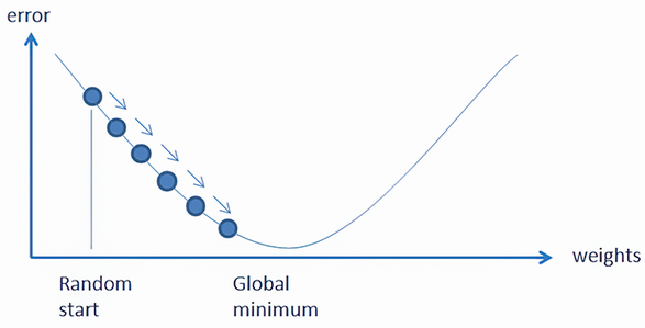
The error surface can be viewed as a landscape: successive gradient-guided steps move from a high-error location toward the lowest valley, the error-function minimum. section 4.3.5
Gradients play distinct practical roles across common tabular-data models:
- In stochastic gradient descent, small batches—or individual streamed examples—supply repeated updates, making learning feasible when data is handled out of core. section 4.3.5
- In regularized linear models, gradients determine coefficient corrections while L1 or L2 penalties constrain the resulting weights. section 4.3.2
- In gradient boosting classification, each iteration fits a regression model to the loss gradient with respect to logits, then improves predictions in the loss-reducing direction. section 5.2.2
Gradient boosting with logits
For classification, probabilities are transformed to logits so the problem can be treated as regression. With squared loss, the gradient corresponds to a residual in logit space; fitting the next model to that gradient progressively improves predictions. Applying the sigmoid converts the final logit prediction back to a value between 0 and 1. section 5.2.2
A gradient supplies local guidance, not a guarantee of the best possible solution. Complex error landscapes can contain local minima and plateaus, and update choices can substantially affect the result. section 4.3.5