A gradient turns the local behavior of a multivariable function into a vector that can guide model training. For a loss L(w) defined over parameters w, the gradient ∇L(w) is the vector containing one partial derivative for each parameter. Each component measures how L changes when that parameter alone is displaced; together, they describe the first-order change in loss under a parameter displacement δw: δL is the dot product ∇L(w)·δw. section 3.0 section 3.3.1
The gradient points in the direction of fastest local increase. Its negative therefore gives the direction of fastest local decrease: for a sufficiently small step, choosing δw proportional to −∇L(w) produces the largest reduction in loss. The gradient is zero at an optimum under the smooth turning-point picture, but a zero gradient can also leave a basic gradient-based update unable to move through a flat region. section 3.3.1 section 8.4.3 section 9.2.4
Figure 3.4 δL in terms of δw in one dimension, illustrated with two example curves: a straight line and a parabola. In general, δL = (dL/dw) δw. To decrease loss, δw must have the opposite sign of the derivative dL/dw. In (a), this implies we always have to move left (decrease w) to decrease L. In (b), if we are in the left half (e.g., point Q), the derivative is negative, and we have to move to the right to decrease L. But if we are in the right half, the derivative is positive, and we have to move to the left to decrease L. Geometrically, this is equivalent to following the tangent “downward.”
|
(a) Line: L(w) = 2w + 1, dL/dw = m |
|
(b) Parabola: L(w) = w2, dL/dw = 2w |
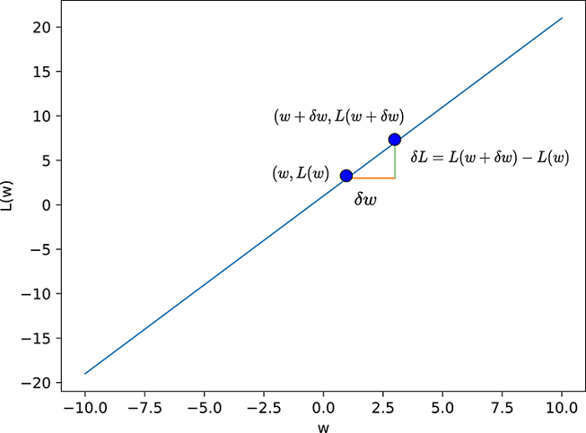
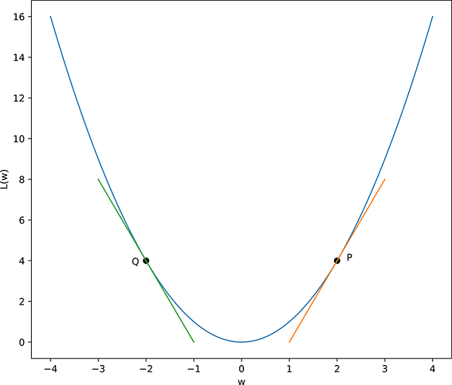
A one-dimensional line and parabola make the sign rule visible: decrease the parameter opposite the derivative to decrease loss. On opposite sides of a parabola’s minimum, the derivative changes sign, so the descent direction changes too. section 3.3.1
Level contours give a geometric view. Moving tangent to a level contour leaves the function value unchanged, whereas the gradient is normal to that contour and points across contours in the direction of greatest increase. Its magnitude corresponds to the magnitude of that change; directions orthogonal to it give zero local change. In three dimensions, the same idea applies to level surfaces such as spheres or cylinders. section 3.3.2
A quadratic loss surface
For L(w0,w1) = 2w0² + 3w1² at (w0,w1) = (3,4), the gradient is [12,24]ᵀ. Many moves lower the loss, but the direction [−12,−24]ᵀ—the negative gradient—gives the maximum reduction locally. The example separates the gradient’s uphill direction from the update used to minimize loss. section 3.3.1
The gradient supplies the first-order term in a multidimensional Taylor approximation. For very small displacements, higher-order terms involving the Hessian become negligible, leaving the gradient-dot-displacement approximation. For somewhat larger displacements, a Hessian term can improve the approximation, though that is noted as rarely used in practice. section 3.4.2
In neural-network training, loss is a function of all weights and biases. Training iteratively adjusts those parameters toward lower loss using their loss gradients, with the learning rate controlling step size. A backward pass computes gradients with respect to weights and biases after a forward pass. Differentiable activations are needed because these gradients are vectors of partial derivatives; a discontinuous Heaviside step function cannot provide them. section 8.1 section 8.4 section 8.6
Practical gradients may be noisy because they are commonly estimated from minibatches. Momentum forms updates from a weighted history of gradients: shared downhill components reinforce while random components tend to cancel. This can also carry updates through a small flat region where a vanilla gradient update would stop. section 9.2.4