A gradient is the vector of partial derivatives describing how a function changes with respect to its parameters. For a neural network, it indicates the direction and rate of steepest increase in the loss. Training therefore moves in the opposite direction, adjusting weights to reduce error. First-order methods use only this local information, avoiding the extra computation of curvature or second-order derivatives. section 2.5.4
Backpropagation computes gradients by multiplying partial derivatives as it moves backward through the layers. If those derivatives are usually below one, the product shrinks with depth and earlier layers receive negligible updates: the vanishing-gradient problem. If they exceed one, gradients can explode, producing erratic updates and preventing convergence. Initialization matters because identical weights give neurons identical gradients, while overly large or small weights can amplify or suppress the signal. section 2.4
Finding the downhill direction
Imagine a hiker who can inspect only a small patch of a foggy mountain. A random mini-batch provides a noisy estimate of the local gradient; the hiker steps opposite that slope. Momentum averages recent steps, reducing jitter and helping movement across shallow plateaus. The learning rate controls the step size: large early steps can become smaller, more deliberate steps near the valley floor. section 2.5.4
Figure 2.2 The challenge of optimizing functions shaped like long, narrow valleys. The contour lines represent a valley, with the optimal direction of progress indicated by an arrow running along the valley’s base. Smaller arrows represent steps taken by gradient descent: the left diagram shows large steps oscillating inefficiently across the valley, while the right diagram shows small steps making slow progress along the base. The “pathological” nature does not arise from high or low curvature, but from the combination of high curvature across the valley and low curvature along it. Used with permission granted by the author (James Martens).
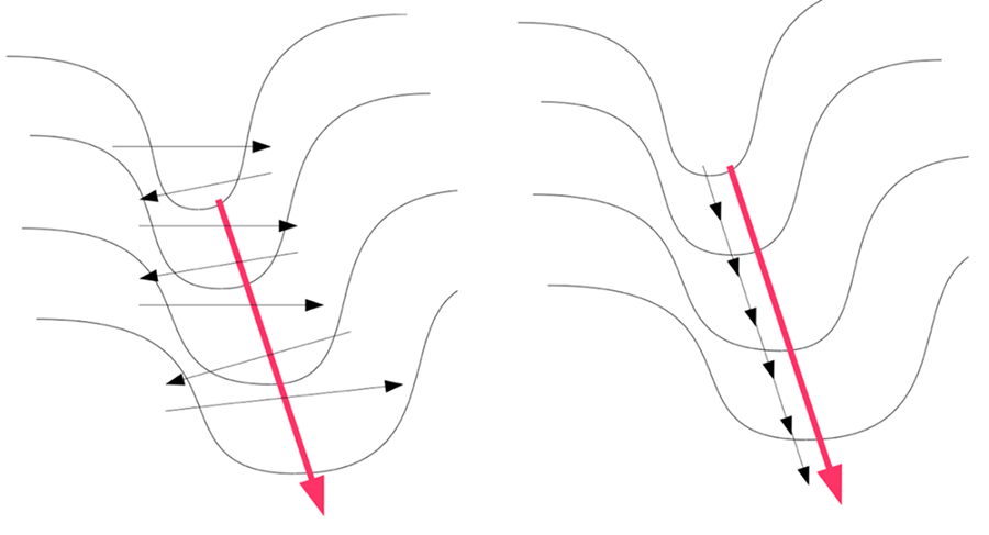
A narrow, curved optimization valley shows why gradient descent can oscillate across a high-curvature direction while progressing slowly along a low-curvature direction. section 2.4
AlexNet used mini-batch stochastic gradient descent with momentum 0.9, batches of 128 images, an initial learning rate of 0.01, and tenfold reductions when validation accuracy stopped improving. These choices illustrate the practical balance among noisy estimates, update size, convergence, memory, and training time. section 2.5.4