A histogram divides a numeric feature’s range into bins and shows how many values fall in each bin. It gives a compact view of the distribution without assuming that values follow a single, roughly Gaussian shape. Sparse bins can identify unusual values at either extreme or between more common groups. section 2.1.6
For outlier detection, choose a bin count, assign each value to a bin, count the values, and flag values in bins judged unusually sparse. For example, an implementation can use pandas `cut()` to make ten equal-width bins and flag bins containing fewer than ten records. Those choices are thresholds, not universal rules: changing the number of bins can change which values are flagged. An empty bin contains no value to flag. section 2.1.6
A gap between common values
Suppose most purchases are near $10 or $500. A rare $100 purchase may be an internal outlier even though it is not an extreme value. A low-count bin between the two groups can expose it; the flag indicates rarity, not that the purchase is illegitimate. section 2.1.6
Figure 2.7 The segment data divided into 10 histogram bins. The x-axis indicates the bins. The height of each bar indicates the number of records in the bin. Dashed vertical lines indicate values flagged as outliers: those in bins with unusually low counts. We can see a number of outliers in bin 4 and in bin 7 (both bins with quite low counts). Bin 6 has no records and so no outliers. This method can identify internal outliers though it is sensitive to the number of bins.
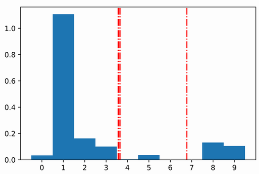
The plotted bins show flagged values in sparse interior bins. One bin is empty, illustrating why a sparse range does not necessarily yield a flagged record. section 2.1.6
Histograms also serve as a visual check. Plotting each numeric column is a useful first step in exploratory data analysis, and marking flagged values on its histogram can help explain one-dimensional outliers. It cannot, by itself, explain a row flagged only because of an unusual combination of features; such values may look ordinary in every individual histogram. section 2.3.2 section 8.1.2
Histogram-based Outlier Score (HBOS) applies the univariate idea across features when speed matters or there are too many features for feasible joint testing. It will miss outliers defined solely by rare feature combinations. For a different task, a histogram can supply bin frequencies and edges for generating synthetic values: sample bin centers according to their frequencies and add jitter. Generating features independently can closely reproduce each column’s distribution while losing associations between columns. section 6.2 section 11.2.2