The learning rate, written η, controls how far an optimization update moves along the direction indicated by the gradient. For a scalar function, gradient descent uses xcur = xcur − η · f′(xcur). section 1.3.3
The gradient identifies which way to move but not how far. A small η takes conservative steps that may require more iterations; an excessive η can overshoot the minimum, bounce around it, or diverge. section 1.3.3
In PyTorch, the learning rate appears directly in either a manual update or an optimizer configuration:
- SGD accepts the parameter list and learning rate through torch.optim.SGD([x_param], lr=eta), then applies updates with optimizer.step(). section 1.4
- Training commonly runs for a fixed number of epochs rather than waiting for zero loss or an imperceptibly small parameter change. section 1.4
- Treating η as a hyperparameter permits automated search with Optuna, alongside choices such as momentum and network architecture. section 5.4
Scalar minimization
Starting with x = −3.5 and η = 0.1, the manual loop repeatedly computes f(x), calls backward(), updates x, and stops when successive guesses change by at most 10⁻⁵. It reaches tensor([2.0000]). section 1.3.3
GAN configuration
A GAN setup uses separate AdamW optimizers for the generator and discriminator, assigning both η = 0.0001 with betas=(0.0, 0.9). section 9.1.3
Figure 1.7 Three examples of how the learning rate η (also called step size) impacts learning. On the left, η is smaller than necessary. This still reaches the minimum but takes more steps than needed. If we knew the perfect value of η, we could set it just right, to take the smallest number of steps to the minimum value (middle). On the right, η is too big, which causes divergence. We never reach the solution!
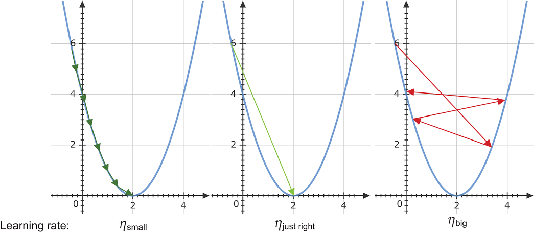
Compare undersized, well-chosen, and oversized learning rates: slower convergence, efficient convergence, and divergence. section 1.3.3
x = torch.tensor([-3.5], requires_grad=True)

x_cur = x.clone()
x_prev = x_cur*100                                  #1

epsilon = 1e-5                                      #2

eta = 0.1                                           #3

while torch.linalg.norm(x_cur-x_prev) > epsilon:
    x_prev = x_cur.clone()                          #4

    value = f(x)                                    #5
    value.backward()
    x.data -= eta * x.grad


    x.grad.zero_()                                  #6


    x_cur = x.data                                  #7

    print(x_cur)

tensor([2.0000])
Trace a complete manual update loop, including gradient computation, the η-scaled parameter update, gradient clearing, and convergence checking. section 1.3.3