Sampling generates random values from a specified probability distribution. Each value is more or less likely according to the distribution’s probability density or mass function. Uniform samples are equally likely, while normal samples cluster near the mean. section 4.1
In Bayesian analysis, a sample represents one possible realization of an uncertain quantity. A collection of samples approximates the distribution that produced them, allowing its shape and summary statistics to be studied. section 4.1 section 5.3
Sampling supports several practical tasks:
- Approximate posterior distributions when conjugacy does not provide a closed-form solution. section 5.0 section 5.3
- Estimate posterior means with sample averages and 95% credible intervals with the 2.5th and 97.5th percentiles. section 5.3
- Generate prior or posterior predictive outcomes for model checking and prediction. section 4.12 section 5.0
From distributions to samples
Drawing 10,000 values from Beta(1, 1) or a normal distribution produces histograms whose shapes approach the corresponding probability density functions. In Python, scipy.stats provides rvs, meaning random variates, for this operation. For an unavailable posterior, Monte Carlo samples similarly provide a usable numerical surrogate. section 4.1 section 5.3
Figure 4.1 True PDFs of Beta(1, 1) and 𝒩(100,100²) (left column) and the corresponding histograms and 10,000 samples drawn from the two probability distributions (right column). Under infinite samples, the shapes of the histograms approach the respective PDFs.
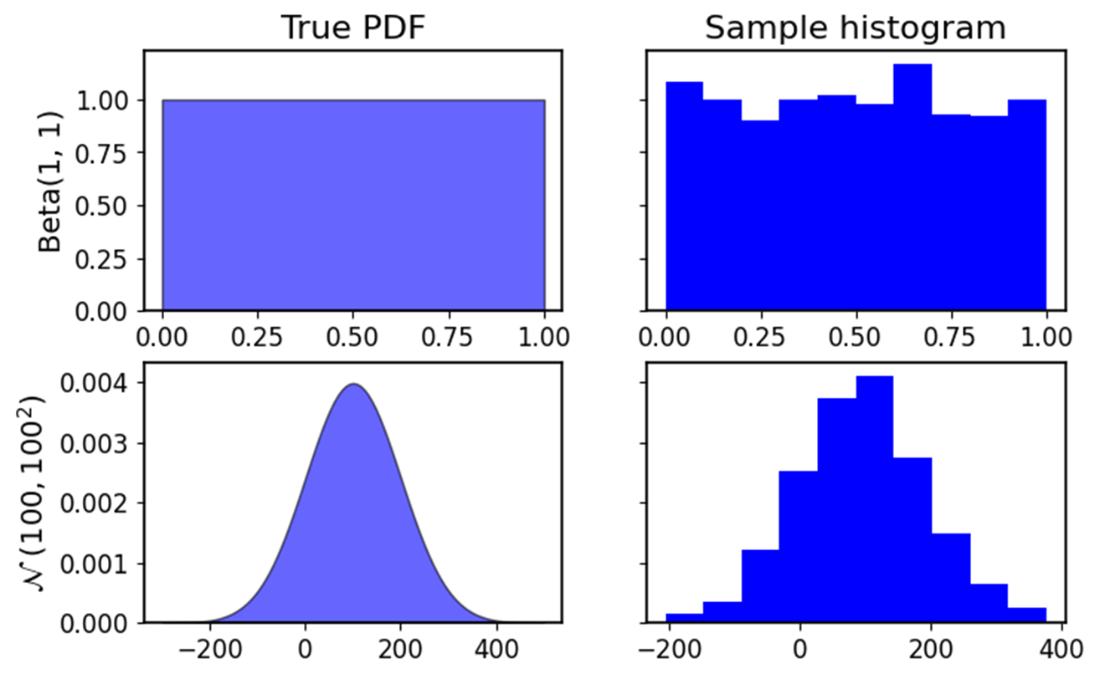
Compare probability density functions with histograms of 10,000 samples to see how sampling reproduces distributional shape. section 4.1
Figure 5.1 Comparison between a posterior distribution available in closed form and Monte Carlo samples. The samples’ histogram matches the true PDF, and the various statistics from the samples give reasonable approximations to the corresponding true quantities.
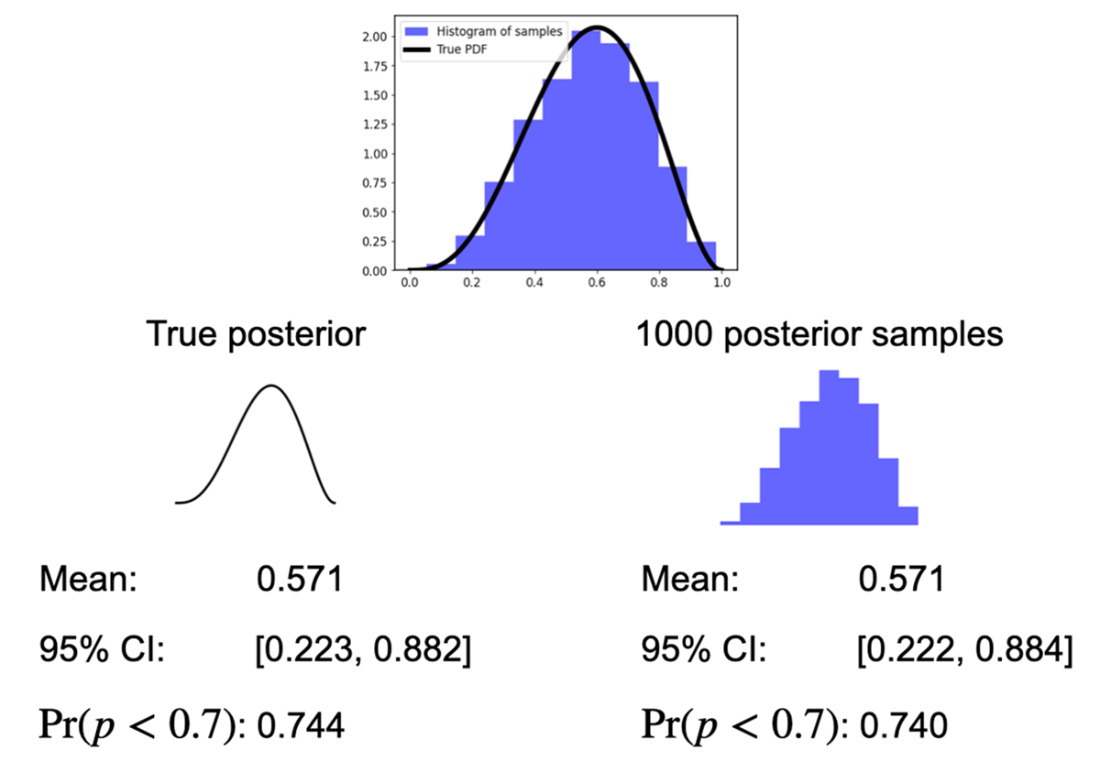
Inspect how posterior samples approximate a known Beta(4, 3) posterior and reproduce its statistics. section 5.3