Slope measures how much a target changes when a predictor increases by one unit. For example, it can represent the change in a house’s price for each additional square foot. section 3.10
A simple linear model writes this relationship as y = mx + b, where m is the slope and b is the intercept. Setting b to zero gives y = mx. A positive slope means predictions increase with x; a negative slope means they decrease. section 3.10
A useful slope is one that keeps predictions close to observed data. In the house-price example, the best value minimizes average squared error and can be calculated directly from historical areas and prices. section 3.10
Bayesian modeling treats the slope as uncertain rather than automatically fixing it at one value:
- A prior distribution expresses beliefs about plausible slopes before observing data. section 3.14
- Observed data update that prior into a posterior distribution, whose mean summarizes the updated slope and whose smaller standard deviation represents reduced uncertainty. section 3.14
- A Normal prior can assign probability to negative house-price slopes, even when domain knowledge says the slope should be non-negative; changing the prior or using sampling can address that mismatch. section 5.2
A changing slope over time
In a CO₂ time series, slope represents the systematic yearly change in concentration. The model lets the slope evolve gradually, treating each year’s slope as similar to the previous year’s while observations remain noisy. Together with the concentration level, it forms a two-variable linear state-space model. section 9.12
Figure 3.5 The prior and posterior distributions of the slope 𝑚. The posterior distribution sharply peaks around the true value 𝑚 = 200 to reflect the insight from the observed data.
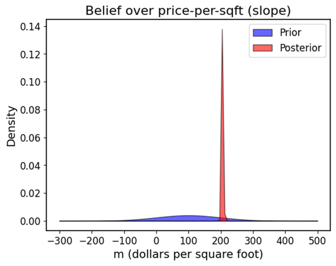
Compare the prior and posterior distributions to see how observed data concentrate belief around a slope near 200. section 3.14
Read the time-series update ℓᵢ₊₁ = ℓᵢ + sᵢ + ε to see how slope contributes to the next concentration level. section 9.12