Autoencoder

As explained in Financial AI in Practice

An autoencoder is a neural network trained to reconstruct its input, typically by encoding it into a lower-dimensional representation and decoding it.

A fraud detector trained on past cases can miss new tactics. An autoencoder offers a complementary way to look for them: it learns to reconstruct legitimate transactions, then treats unusually poor reconstructions as potential anomalies. It does not establish that a transaction is fraudulent; it identifies candidates for further review. section 8.4 section 8.4.1

Figure 8.9 Autoencoder architecture for unsupervised fraud detection. The encoder compresses the input transaction X into a low-dimensional representation h, and the decoder reconstructs it as X-hat. Anomalous (potentially fraudulent) transactions are identified when the reconstruction error |X – X-hat|₂ is significantly high, indicating patterns the model didn’t learn during training on normal data.

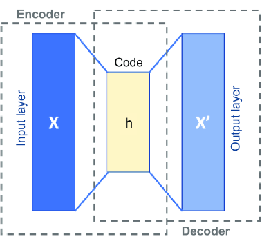
The encoder compresses transaction features into a smaller representation; the decoder reconstructs the original features. A large difference between input and reconstruction signals a pattern the model did not learn well. section 8.4.1

A practical credit-card workflow separates learning normality from testing whether the score is useful:

• Start with scaled training and test features. Filter the training features to legitimate transactions (`X_train[y_train == 0]`); labels select normal examples but are not reconstruction targets. section 8.4.2
• Build a symmetric Keras autoencoder with Dense layers, BatchNormalization, LeakyReLU, and a lower-dimensional bottleneck. Use a linear output because standardized features can be negative or positive; check the compression and expansion with `model.summary()`. section 8.4.3
• Train on legitimate transactions as both inputs and targets. Validate on a separate legitimate subset; inspect training and validation loss, and use early stopping to restore the best weights. section 8.4.3
• Reconstruct the full test set and compare errors for legitimate and fraudulent transactions. Mean squared error or mean absolute error can serve as the anomaly score. section 8.4.1 section 8.4.2

Turning scores into alerts requires an operational threshold, not just a model fit. Examine normal-error statistics and class separation where test labels exist, then account for analyst review capacity and customer friction. Shadow-mode testing with analyst feedback can inform the threshold before live decisions; real-time use also requires serving, feature retrieval, logging, and monitoring. section 8.5

How Financial AI in Practice covers it

How deep it goes

Works through data filtering, architecture, training, error-based evaluation, and threshold considerations; it does not supply a universal alert threshold.

Examples

Uses scaled credit-card transactions, a Keras encoder–decoder, legitimate-only training, and a mixed legitimate-and-fraudulent test set.

What it assumes

Assumes prepared, scaled training and test features and known legitimate training examples; defines self-reconstruction and anomaly scoring in plain language.

What you can do after

Build it from scratch with Keras to score transaction anomalies, then evaluate errors and choose a review threshold with operational feedback.

How it connects

Connects unsupervised anomaly detection to reconstruction error, supervised fraud classification, and operational alert thresholds.

liveBookmanning.com

Read Financial AI in Practice on liveBook Get the book at manning.com

Also explained in

• 

  liveBookmanning.com
  Inside Deep Learning: Math, Algorithms, ModelsA neural network trained to reconstruct its input, typically by compressing it into a lower-dimensional latent representation and decoding it back.
• 

  liveBookmanning.com
  Outlier Detection in PythonAn autoencoder is a neural network trained to encode an input into a representation and reconstruct the original input.
• 

  liveBookmanning.com
  Math and Architectures of Deep LearningA neural network model trained to compress inputs into a latent representation and reconstruct the original inputs from that representation.
• 

  liveBookmanning.com
  Data Without LabelsAn autoencoder is a neural-network model that learns to encode data into a lower-dimensional representation and reconstruct the original input from it.
• 

  liveBookmanning.com
  Evolutionary Deep Learning: Genetic algorithms and neural networksAn autoencoder is a neural network that learns to encode inputs into a representation and decode that representation to reconstruct the inputs.
• 

  liveBookmanning.com
  Learn Generative AI with PyTorchA neural network that learns to compress inputs into a latent representation and reconstruct them, used here for digit-image generation and reconstruction.
• 

  liveBookmanning.com
  Graph Neural Networks in ActionAn autoencoder is a neural network that encodes inputs into latent representations and decodes those representations to reconstruct the inputs.
• 

  liveBookmanning.com
  Delivering Machine Learning Projects: From design to deploymentAn autoencoder is a neural network that learns to encode inputs into a lower-dimensional representation and reconstruct the original inputs.
• 

  liveBookmanning.com
  Deep Learning with R, Third EditionAn autoencoder is a neural-network model that learns to encode inputs into representations and decode those representations back into approximations of the inputs.
• 

  liveBookmanning.com
  Deep Learning with Python, Third EditionA neural network trained to reconstruct its input, often by compressing and then decoding it, used here for denoising images.
• 

  liveBookmanning.com
  Introduction to Generative AI, Second EditionAn autoencoder is a neural network that learns to encode data into a compressed representation and reconstruct the original data from it.

Compare how 12 books explain autoencoder →

Related concepts

• encoderhas part · An encoder is a component that transforms input data into an encoded representation for subsequent processing, reconstruction, comparison, or transmission.
• decoderhas part · A decoder is a component that maps encoded data or representations to decoded values, reconstructed data, or generated output.
• variational autoencoderincludes · A variational autoencoder is a generative neural network that learns a probabilistic latent representation of data and decodes samples from it to reconstruct or generate data.
• deep learningkind of · Deep learning is a machine-learning approach that uses neural networks with multiple computational layers to learn representations from data.
• neural networkkind of · A neural network is a computational model of interconnected, parameterized units that learns transformations from inputs to outputs.
• Kerasuses · Keras is an open-source, high-level deep-learning API for building, training, evaluating, and deploying neural-network models.

This explainer was generated by Manning's knowledge graph from the text of Financial AI in Practice. The section links point to the parts of the book it draws on.