Autoencoder

As explained in Inside Deep Learning: Math, Algorithms, Models

A neural network trained to reconstruct its input, typically by compressing it into a lower-dimensional latent representation and decoding it back.

An autoencoder learns to reproduce an input without human-provided labels. It combines an encoder f_in(x) = z, which creates a latent representation, with a decoder f_out(z) = x̂, which reconstructs the input. Training minimizes reconstruction error while constraining the network so it cannot simply copy x unchanged. section 7.0 section 7.1

A practical autoencoder design follows these choices:

• Use a bottleneck whose layers shrink toward a latent dimension D′, then expand symmetrically through the decoder. The bottleneck prevents the naive identity solution. section 7.2
• Train fully connected implementations with mean squared error; flatten image inputs such as (B, 1, 28, 28) before linear layers and reshape decoded outputs afterward. section 7.2.1
• Add nonlinear layers such as ReLU and batch normalization to move beyond linear PCA, or share encoder weights with transposed decoder layers when reproducing PCA-like behavior. section 7.1.2 section 7.1.5
• Inject Gaussian or dropout noise during training while retaining the clean input as the reconstruction target; disable training-time perturbation during evaluation. section 7.3.1 section 7.4.1

MNIST bottleneck autoencoder

For 28×28 grayscale images, set D = 28×28 and choose a two-dimensional latent space. An encoder can flatten the image and reduce D → D/2 → D/3 → D/4 → 2; a decoder reverses those sizes and reshapes its D outputs to (1, 28, 28). Train the combined network with MSE, then plot the two latent coordinates and inspect reconstructed digits. Increasing the latent size can preserve more detail, but reconstruction quality alone does not prove that the representation is useful. section 7.2.1 section 7.3

Denoising and outlier detection

A denoising autoencoder adds sampled noise s ~ N(0, 0.5) to create x̃ = x + s, then learns to reconstruct clean x. For anomaly detection, compute reconstruction errors and review examples above a chosen threshold, such as the highest 0.1% of errors. section 7.3.1 section 7.2

Figure 7.2 The process of autoencoding. The input goes through an encoder that produces a new representation of the data z. The representation z can be useful for lots of tasks like clustering, search, and even classification. The decoder attempts to reconstruct the original input x from the encoding z.

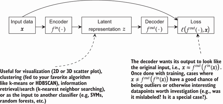
Use the encoder–latent–decoder diagram to trace how an input becomes a compact representation and returns as a reconstruction. section 7.1

How Inside Deep Learning: Math, Algorithms, Models covers it

How deep it goes

Explains latent representations, bottlenecks, noise constraints, PCA connections, and PyTorch implementations, but defers sequence cases to autoregressive models.

Examples

Uses MNIST digit reconstructions, two-dimensional latent plots, PCA implementations, Gaussian noise, dropout noise, and reconstruction-error thresholds.

What it assumes

Assumes familiarity with neural-network regression, loss functions, PyTorch modules, tensors, and basic dimensionality reduction.

What you can do after

Builds fully connected PyTorch autoencoders, trains them with MSE, inspects reconstructions, and evaluates robustness or outliers.

How it connects

Connects self-supervision with PCA, dimensionality reduction, denoising, outlier detection, clustering, search, and classification.

liveBookmanning.com

Read Inside Deep Learning: Math, Algorithms, Models on liveBook Get the book at manning.com

Also explained in

• 

  liveBookmanning.com
  Outlier Detection in PythonAn autoencoder is a neural network trained to encode an input into a representation and reconstruct the original input.
• 

  liveBookmanning.com
  Math and Architectures of Deep LearningA neural network model trained to compress inputs into a latent representation and reconstruct the original inputs from that representation.
• 

  liveBookmanning.com
  Data Without LabelsAn autoencoder is a neural-network model that learns to encode data into a lower-dimensional representation and reconstruct the original input from it.
• 

  liveBookmanning.com
  Evolutionary Deep Learning: Genetic algorithms and neural networksAn autoencoder is a neural network that learns to encode inputs into a representation and decode that representation to reconstruct the inputs.
• 

  liveBookmanning.com
  Learn Generative AI with PyTorchA neural network that learns to compress inputs into a latent representation and reconstruct them, used here for digit-image generation and reconstruction.
• 

  liveBookmanning.com
  Graph Neural Networks in ActionAn autoencoder is a neural network that encodes inputs into latent representations and decodes those representations to reconstruct the inputs.
• 

  liveBookmanning.com
  Delivering Machine Learning Projects: From design to deploymentAn autoencoder is a neural network that learns to encode inputs into a lower-dimensional representation and reconstruct the original inputs.
• 

  liveBookmanning.com
  Financial AI in PracticeAn autoencoder is a neural network trained to reconstruct its input, typically by encoding it into a lower-dimensional representation and decoding it.
• 

  liveBookmanning.com
  Deep Learning with R, Third EditionAn autoencoder is a neural-network model that learns to encode inputs into representations and decode those representations back into approximations of the inputs.
• 

  liveBookmanning.com
  Deep Learning with Python, Third EditionA neural network trained to reconstruct its input, often by compressing and then decoding it, used here for denoising images.
• 

  liveBookmanning.com
  Introduction to Generative AI, Second EditionAn autoencoder is a neural network that learns to encode data into a compressed representation and reconstruct the original data from it.

Compare how 12 books explain autoencoder →

Related concepts

• encoderhas part · An encoder is a component that transforms input data into an encoded representation for subsequent processing, reconstruction, comparison, or transmission.
• decoderhas part · A decoder is a component that maps encoded data or representations to decoded values, reconstructed data, or generated output.
• variational autoencoderincludes · A variational autoencoder is a generative neural network that learns a probabilistic latent representation of data and decodes samples from it to reconstruct or generate data.
• deep learningkind of · Deep learning is a machine-learning approach that uses neural networks with multiple computational layers to learn representations from data.
• neural networkkind of · A neural network is a computational model of interconnected, parameterized units that learns transformations from inputs to outputs.
• Kerasuses · Keras is an open-source, high-level deep-learning API for building, training, evaluating, and deploying neural-network models.

This explainer was generated by Manning's knowledge graph from the text of Inside Deep Learning: Math, Algorithms, Models. The section links point to the parts of the book it draws on.