A bar chart, also called a bar graph, compares discrete categories with rectangular bars. Each category or factor receives one bar, and its length encodes a count, frequency, or supplied value. Bars are commonly vertical, but horizontal bars can improve readability when category labels are long. section 1.2.1 section 2.5.5
Use a bar chart to answer a categorical comparison question: Which group has more? Which segment has the higher average? What changed across seasons or quarters? It is especially useful after reducing messy records into a grouped summary, such as mean win shares by birthplace or average games played by draft-pick segment. section 2.5.5 section 3.5.1
Build a meaningful bar chart in R with a deliberate sequence:
- Group and summarize the data when the bar should represent a statistic such as a mean, median, percentage, or average rather than raw records. section 2.5.5 section 14.3
- Map the category to x and the prepared numeric result to y, then use geom_bar(stat = "identity") so bar lengths match those supplied y values. section 3.5.1 section 14.3
- Omit stat = "identity" when the intended result is the count of records in each x category; otherwise ggplot2 counts x values by default. section 3.5.1 section 14.3
- Control category order explicitly when default ordering is misleading, and use coord_flip() for a horizontal ranking. section 3.5.1 section 11.4.2
- Add labels with geom_text() or geom_label(), leaving enough axis space with ylim() or xlim() so labels remain visible. section 2.5.5 section 3.5.1
Compare career win shares by birthplace
First, group NBA draft records by birthplace and compute mean and median career win shares. Then draw one identity bar chart for each statistic, label the truncated values, and keep both y-axes on the same 0–35 scale. Matching scales matter: different scales could make unequal values appear equal-height. The resulting comparison shows higher mean and median career win shares for USA-born players than for players born elsewhere. section 2.5.5
Bar charts can make an analytical claim easier to inspect when styling supports the question. For quarter-by-quarter win percentages, a highlighted bar can direct attention to the standout quarter while subdued bars retain the comparison. For many subsets, faceting creates one small bar chart per condition, with shared scales helping comparisons across panels. section 6.4.5 section 9.5.2
Test whether games are won in the fourth quarter
A pair of bar charts compares how often winning a quarter coincides with winning the game, including home and road splits. The fourth-quarter winner also won the game in nearly 66% of applicable games, but the third quarter produced a higher association overall. The chart therefore challenges, rather than merely illustrates, the claim that games are won in the fourth quarter. section 6.4.4 section 6.4.5
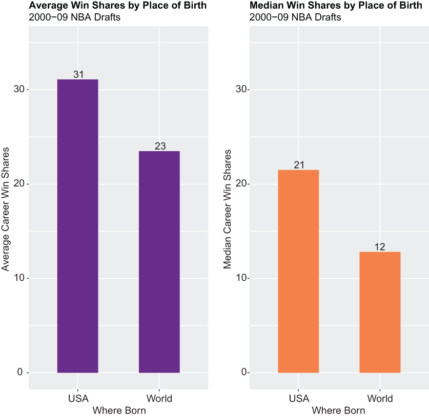
Compare the paired mean and median bars on a shared scale to see how the same categories can support two different summary measures. section 2.5.5