A directed acyclic graph (DAG) is a causal model in which variables are nodes and arrows represent causal relationships. “Directed” means an arrow from A to B says changing A affects B, not vice versa. “Acyclic” means following arrows never leads back to the starting node. DAGs turn a causal question into an explicit map of how data may have been generated. section 1.1.3 section 3.1
Use a DAG before choosing an estimation method. Drawing the graph makes assumptions visible, identifies relevant observed and unobserved variables, and specifies the treatment, outcome, and causal effect of interest. Its geometry determines later calculations, including whether adjustment for confounding is needed. section 3.0 section 3.1
A useful causal DAG distinguishes several roles variables can play:
- Treatment and outcome: the proposed cause and effect, linked by the causal effect being estimated. section 1.8 section 10.2.1
- Confounders: variables that influence both treatment and outcome, creating paths that can make correlation misleading. section 1.1.3 section 1.8
- Mediators: variables lying on a causal route between treatment and outcome. section 1.1.3 section 3.2.2
- Colliders and other path structures: variables whose conditioning can open or close correlation paths, affecting which adjustments are valid. section 7.8
Topic, pageviews, and hidden common causes
To estimate the effect of a webpage topic on pageviews, draw Topic → Pageviews, then add variables supported by domain knowledge. Seasonality and popularity can be confounders when they affect both topic and pageviews; platform can be a mediator. The diagram does not prove these arrows from data alone—it records assumptions that guide what to adjust for. section 3.2.2 section 7.8
A DAG is not discovered automatically from correlations. The same paired data can fit causal models with opposite arrow directions, so domain expertise is essential. Missing a relevant confounder can undermine a causal conclusion; conversely, a graph should also state meaningful absences of arrows rather than silently assuming them away. section 3.2.2 section 2.9
Figure 3.7 Graph representing pricing discounts based on historical purchasing frequency. Price and demand affect future prices and demands.
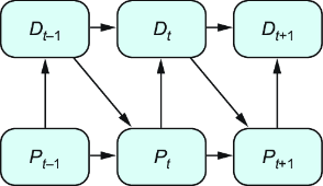
Feedback can appear cyclic when price changes demand and demand later changes price. Representing variables at successive time points, such as Price at t → Demand at t → Price at t+1, can unfold this process into an acyclic graph. section 3.2.2
DAGs support graphical causal inference: d-separation and the back-door criterion use the graph to determine which variables to condition on before applying an adjustment formula. The same causal ideas can also be expressed in the potential-outcomes framework; an intervention in a DAG corresponds to a potential outcome through the do operator. section 7.8 section 10.2.1
The acyclic requirement is a real limitation. Simultaneous reciprocal causation cannot be represented by an ordinary DAG unless it can be unfolded over time; without suitable time-series data, the graphical approach may be difficult to apply. A graph is useful only insofar as its assumptions fit the decision and setting at hand. section 3.2.2 section 1.1.3