A gradient is a vector of partial derivatives of a scalar function. Each component measures how the function changes as one variable changes. The gradient points toward the steepest increase; the negative gradient points downhill. section 4.2.3 section 8.2.1
In model training, the scalar function is often a loss: a measure of how far predictions are from their targets. The gradient of the loss with respect to each weight or bias indicates how that parameter affects the loss. Gradient descent updates parameters in the negative-gradient direction, using a learning rate to control step size. section 4.2.3 section 8.2.1
Predicting EGFR activity
A neural network takes a molecule’s 2,048-bit Morgan fingerprint as input and predicts its pIC50 against EGFR. Mean squared error compares the prediction with the measured value; gradients indicate how to adjust the network’s weights to reduce that loss. section 8.2
A forward pass computes a prediction and its loss. Backpropagation then applies the chain rule backward through the computational graph, combining local derivatives to calculate the loss gradient for each trainable parameter. section 8.2.1
Listing 8.5 Logistic Regression Model Class
x = torch.tensor([1.0, 2.0, 3.0])
w = torch.tensor([0.1, 0.2, 0.3], requires_grad=True)
b = torch.tensor(0.1, requires_grad=True)

z = torch.sum(x * w) + b
y = torch.sigmoid(z)

target = torch.tensor(1.0)
loss = torch.binary_cross_entropy(y, target)

loss.backward()
print(f"Gradient of w: {w.grad}")
print(f"Gradient of b: {b.grad}")
This PyTorch example marks weights and bias as trainable, calls loss.backward(), and prints their gradients. section 8.2.1
A typical PyTorch training step uses gradients in this order:
- Call optimizer.zero_grad() to reset parameter gradients, then compute predictions and loss for the current batch. section 8.2.3
- Call loss.backward() to compute gradients, then optimizer.step() to update parameters. section 8.2.3
- During validation, use model.eval() and torch.no_grad(); calculate loss without updating parameters. section 8.2.3
Batch gradient descent uses the full training dataset to calculate each gradient. Stochastic gradient descent instead uses individual examples or small batches, trading a noisier update for better scaling. A small gradient alone is not always a sufficient stopping signal: combining an iteration limit with cost and improvement thresholds helps avoid stopping at a plateau. section 4.2.3
Figure 4.12 A combination of gradient descent stopping criterion works best to mitigate early termination when hitting the first plateau.
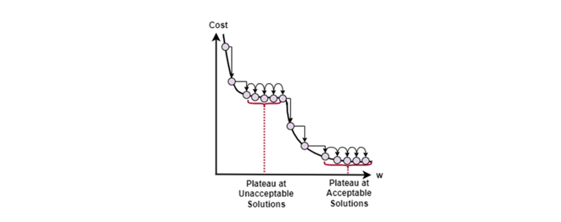
The stopping-criteria figure illustrates why a plateau calls for more than one termination check. section 4.2.3