Probability assigns a likelihood to each possible measurement outcome. In a quantum computation, the state carries one probability for every outcome; repeated executions produce outcome frequencies that approach those encoded probabilities. A single run still returns only one outcome, so probability describes expected distributions rather than a prediction of an individual measurement. section 1.4.2 section 3.4
Figure 1.8 The stages of a computation with a probabilistic bit. In this example, the initial probability that the outcome will be tails is 0.7. During the computation, the probability that the outcome will be tails is changed to 0.3. For example, each time the same computation is repeated (the coin is tossed), we get one outcome according to these encoded probabilities. If we perform 10 repetitions (tosses), we expect to see roughly 7 heads and 3 tails. The more tosses we perform, the closer we expect the distribution of outcomes to be to the encoded probabilities.
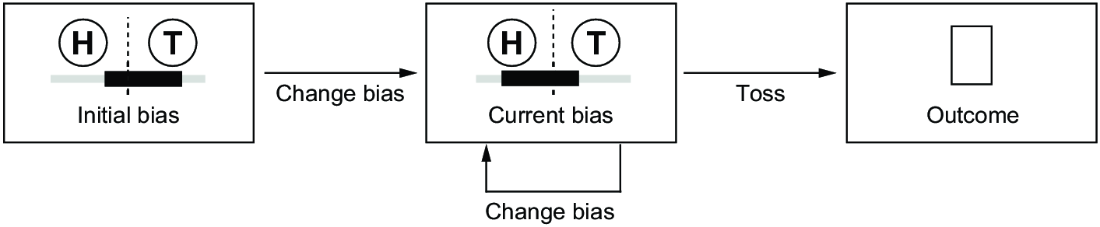
Use the variable-bias coin as a developer-friendly model: computation changes an outcome distribution, while each measurement samples one result from it. section 1.4.2
Quantum probabilities are derived from amplitudes, not stored independently. Each outcome has a complex amplitude with magnitude and direction; its probability is the squared magnitude, p = |z|². Directions do not directly determine measurement frequency, but they matter when gates recombine amplitudes and thereby change later probabilities. Valid state probabilities add to 1. section 2.2.2 section 4.2.2
Represent and inspect outcome probabilities with a state table:
- Map each list index to its corresponding outcome and store that outcome’s complex amplitude. section 3.1.3
- Compute magnitude with abs(amplitude), then square it to obtain the probability. section 3.1.3
- Display amplitude, direction, magnitude, and probability together when debugging or explaining a state. section 3.1.1
Sampling a single-qubit distribution
A state can assign probabilities 0.71651 to outcome 0 and 0.28349 to outcome 1. Sampling ten measurements may yield seven 0s and three 1s; sampling 1,000 times produces counts closer to the distribution. In Python, pass the outcomes and their squared amplitude magnitudes as weights to random.choices, then count the samples. section 3.4
For n qubits, there are 2ⁿ binary-string outcomes, each with a probability. A uniform distribution gives every outcome equal probability and can be prepared by applying a Hadamard gate to every qubit in a default three-qubit state. More generally, gates alter amplitudes in pairs, changing the resulting probability distribution. section 4.3.4 section 4.2.2
Probability can encode an answer rather than a single digital result. Analog encoding uses the probability of one outcome, or the combined probability of several outcomes; estimating it requires many repeated preparations and measurements, called shots. Optimization and search procedures instead aim to increase the probability of desired outcomes before measurement. section 1.5.3 section 2.5
Amplifying good outcomes with Grover iteration
Grover iteration tracks the combined measurement probability of outcomes selected by a predicate. Starting from a uniform state, repeated oracle-and-inversion steps increase the amplitude—and therefore probability—of good outcomes for an appropriate number of iterations. A classical implementation can sum abs(state[k])**2 over selected indices to assert the combined probability. section 6.1.4