What is the chance that it will snow today? Without knowing where you are or the time of year, you can only make a vague estimate. Each useful detail can change that estimate. Probability gives a number to the likelihood of an event; conditional probability asks how likely it is once some information is known. section 8.0
A probability changes with new information
Suppose you are guessing whether an animal is a dog. Learning that it is a house pet raises your estimate; learning that it has wings makes the estimate zero. The notation P(A|B) means “the probability of A given B.” For instance, P(rain today | living in the Amazon rain forest) = 0.8 says that the chance of rain under that condition is 80%. section 8.0 section 1.1
Bayes’ theorem formalizes how information changes a probability. This matters in classification: if you can estimate the probability of a positive label given an item’s features, you can use that estimate to predict its label. A naive Bayes classifier applies this idea to tasks such as deciding whether an email is spam from its words. section 8.0
The clerk in the red sweater
Aisha works three days a week and Beto two, so before looking inside, the chance of finding Aisha is 3/5. Aisha wears red on one-third of her workdays; Beto wears it on half of his. Seeing a red sweater changes the question: among occasions when the clerk wears red, how often is that clerk Aisha? The two possibilities contribute equally—(3/5)(1/3) and (2/5)(1/2)—so the revised probability is 1/2. Try working through the same question before checking the arithmetic. section 8.5
Probability also helps compare classifiers. A logistic classifier predicts a number between 0 and 1 rather than only a label. Log loss penalizes it according to the probability it assigned to the correct label: confident mistakes receive a larger penalty than predictions that give the correct label a high probability. section 6.6
For a decision-tree split, probability can measure how mixed each resulting group is. Imagine drawing two balls, allowing the same ball to be drawn twice. The Gini index is the probability that their colors differ: if color i accounts for a fraction pi of the group, Gini = 1 − p1² − p2² − … − pn². A mostly one-color group has a lower index than a group with many colors. Comparing the groups’ indices helps choose a split. section 9.2
Figure 9.11 The calculation of the Gini index for the set with eight black balls and two white balls. Note that if the total area of the square is 1, the probability of picking two black balls is 0.82, and the probability of picking two white balls is 0.22 (these two are represented by the shaded squares). Thus, the probability of picking two balls of a different color is the remaining area, which is 1 – 0.82 – 0.22 =0.32. That is the Gini index.
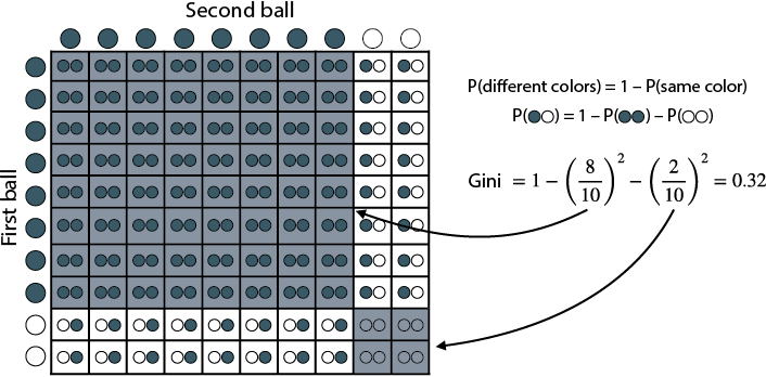
The shaded squares show the same-color outcomes. The remaining area is the probability of different colors: 1 − 0.8² − 0.2² = 0.32. section 9.2
To practice, use the patient symptom table to estimate a diagnosis with naive Bayes. Treat any symptom not mentioned in a question as unknown—not as absent. Then ask which observations actually change your estimate. section 8.5