An objective function turns training into a quantitative problem: it assigns a loss, or penalty, to a model’s output and parameters. In supervised learning, the loss for one input measures the mismatch between a prediction and its known ground truth; total training loss combines those losses across the training set. Training seeks weights and biases that minimize that total. section 9.1 section 9.1.1
For a model output y and target ȳ, mean squared error uses the squared difference (y − ȳ)². Squaring makes positive and negative errors equally costly, and summing individual losses makes the objective reflect performance over the whole training set rather than a few favorable cases. section 3.2 section 8.4 section 1.8
Classification probabilities
For cat, dog, airplane, and automobile classification, cross-entropy compares a one-hot ground-truth distribution with predicted class probabilities. A prediction concentrated on the correct class has lower loss than a uniform, mismatched prediction; the illustrated values are 0.22 for a good prediction and 1.38 for a bad one. section 6.3
An objective can be viewed as a surface over parameter space: each choice of weights and biases has a height equal to its loss. The gradient identifies the direction of greatest increase, so stepping along the negative gradient reduces loss most rapidly locally. Gradients must be recomputed after each update because the surface slope changes with the parameters. section 3.3.1 section 8.4.2
Figure 3.4 δL in terms of δw in one dimension, illustrated with two example curves: a straight line and a parabola. In general, δL = (dL/dw) δw. To decrease loss, δw must have the opposite sign of the derivative dL/dw. In (a), this implies we always have to move left (decrease w) to decrease L. In (b), if we are in the left half (e.g., point Q), the derivative is negative, and we have to move to the right to decrease L. But if we are in the right half, the derivative is positive, and we have to move to the left to decrease L. Geometrically, this is equivalent to following the tangent “downward.”
|
(a) Line: L(w) = 2w + 1, dL/dw = m |
|
(b) Parabola: L(w) = w2, dL/dw = 2w |
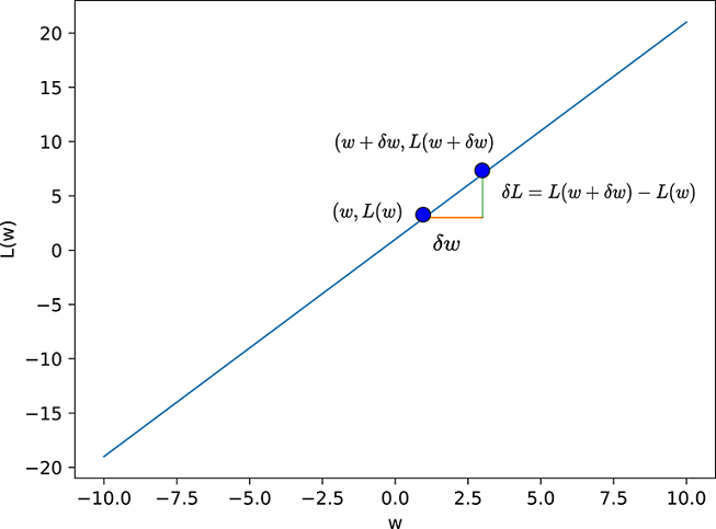
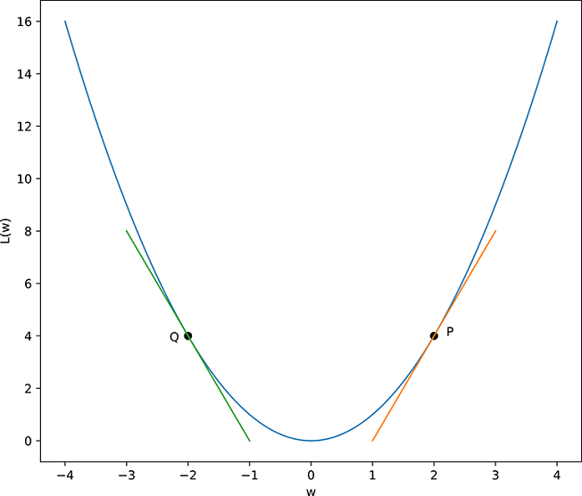
Use the line and parabola to see how the derivative’s sign determines the parameter change that lowers a one-dimensional objective. section 3.3.1
Objective functions are selected to match what a model must make similar:
- Use mean squared error as a representative mismatch between neural-network outputs and ground truth. section 8.4
- Use cross-entropy when outputs are class probabilities and targets select the correct class. section 6.3
- Use binary cross-entropy to compare normalized image or vector tensors, including an autoencoder’s reconstruction against its input. section 9.1.4
- Combine classification cross-entropy with smooth L1 regression loss for Fast R-CNN object regions; only object regions contribute to regression loss. section 11.4.3
Minimizing training loss does not guarantee the best possible parameters: optimization can stall at a local minimum, and satisfactory test-data results are used to judge when to stop. If results are inadequate, changing training data, the loss function, architecture, or random initialization are possible responses. section 8.4