A sigmoid maps an unrestricted numerical score to a value between 0 and 1. The logistic sigmoid is σ(z) = 1 / (1 + e^(−z)), where z is the input score and e is approximately 2.72. Its S-shaped curve has a midpoint at z = 0, where σ(z) = 0.5. section 3.3.2 section 11.3.2
Figure 3.2 The logistic (sigmoid) function maps the linear predictor onto a probability between 0 and 1. The midpoint occurs at 𝑧 = 0, corresponding to a predicted probability of 0.5.
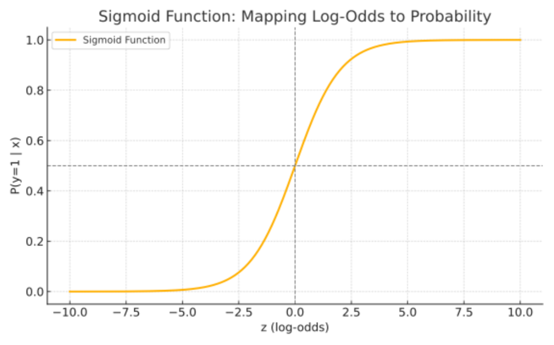
The curve shows how the logistic function maps a linear predictor to a probability, with a midpoint of 0.5. section 3.3.2
In logistic regression, the input is the linear predictor z = β₀ + β₁x₁ + ⋯ + βₖxₖ. Here β₀ is the intercept, βᵢ are coefficients, and xᵢ are predictor variables. The linear predictor represents the log-odds of the positive outcome; the sigmoid transforms it into the predicted probability of that outcome. section 3.3.2
From score to probability
With z = −6 + 1.2x, an input of x = 5 gives z = 0 and a predicted probability of 0.50. Inputs of x = 2 and x = 8 give probabilities of approximately 0.027 and 0.973, respectively. section 3.3.2
In a neural network, sigmoid activation can also transform hidden-node pre-activation values into internal signals. These values are not probabilities, even though they lie between 0 and 1. The nonlinear transformation prevents the network from collapsing into a single linear calculation; the sigmoid's straightforward derivative also simplifies backpropagation calculations. section 11.3.2
Hidden-node activation
For an input of 2.0, two hidden nodes with pre-activation values 1.1 and 0.1 produce sigmoid outputs of approximately 0.75 and 0.52. These outputs form a hidden-layer representation passed to the output node, whose sigmoid output can represent a positive-class probability. section 11.3.2