Decision tree

As explained in Statistics Slam Dunk

A decision tree is a predictive model that recursively partitions data using feature-based decision rules.

A decision tree regression predicts a continuous outcome by dividing data into regions with a series of if-else rules. Each split uses a predictor value, and the endpoint of each branch supplies a predicted value for that subset. Because the result is drawn as an upside-down tree, it can be easier to interpret and explain than a linear regression. section 5.0 section 5.8

Read the tree from top to bottom. Early splits are more significant than splits near the bottom, while terminal nodes, or leaves, are the endpoints where predictions are attached. A tree need not use every candidate predictor, even when all are included in the model formula. section 5.8

Fit and inspect a regression tree in R:

• Load the tree package, then fit a model with tree(), using a continuous target and selected predictors. section 5.1 section 5.8
• Call summary() to inspect terminal-node count and residual mean deviance; its square root is a rough average prediction difference. section 5.8
• Call plot() and text() to visualize the splits and predicted values as a tree. section 5.8
• Compare the tree’s selected predictors with results from a linear regression when checking whether both models identify similar influential variables. section 5.9

Which hustle statistics relate to wins?

Regular-season wins are modeled from points off screens, deflections, loose balls recovered, contested two-point shots, and contested shots. The fitted tree produces 10 terminal nodes and highlights points from screens, deflections, and loose balls recovered as more influential than the other hustle measures. Its rules yield predicted wins for each region of the data. section 5.8 section 5.9

Figure 5.16 The visualized results of our regression tree

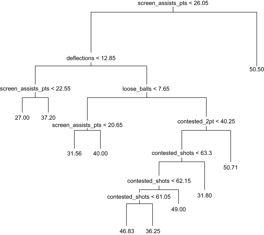
Use the plotted tree to trace the major predictor splits from the root to terminal predictions. section 5.8

Trees trade some accuracy for clarity: a single regression tree can be relatively easy to build and explain but may be less accurate than other supervised-learning methods. Bagging, random forests, and boosting address this by combining many trees into one prediction. section 5.8

For a binary target, the same tree() syntax can fit a classification tree rather than a regression tree. The key distinction is the target: regression trees use continuous outcomes, while classification trees require binary outcomes. section 5.9

How Statistics Slam Dunk covers it

How deep it goes

Explains predictor splits, terminal nodes, residual error, fitting, and visualization without detailing the tree-building algorithm.

Examples

Models NBA regular-season wins from screen points, deflections, loose balls, and contested-shot statistics.

What it assumes

Assumes prepared training data, a continuous target, and predictor variables before fitting the model.

What you can do after

Apply it via R's tree() function to fit and visualize continuous-outcome prediction rules.

How it connects

Connects decision trees with multiple linear regression, classification trees, bagging, random forests, and boosting.

liveBookmanning.com

Read Statistics Slam Dunk on liveBook Get the book at manning.com

Also explained in

• 

  liveBookmanning.com
  Grokking Machine LearningAn algorithm that recursively splits labeled data using feature tests and stopping conditions to construct a decision tree.
• 

  liveBookmanning.com
  Statistics Every Programmer NeedsA decision tree is a graphical decision-analysis model that represents choices, uncertain events, possible outcomes, probabilities, and payoffs as branching paths.
• 

  liveBookmanning.com
  Machine Learning for Tabular Data: XGBoost, Deep Learning, and AIA decision tree is a predictive model that recursively partitions inputs using feature-based split rules and produces outcomes at terminal leaves.
• 

  liveBookmanning.com
  Ensemble Methods for Machine LearningA decision tree is a predictive model that recursively partitions data according to feature-based decisions, producing predictions at the resulting leaves.
• 

  liveBookmanning.com
  Outlier Detection in PythonA decision tree is a hierarchical predictive model that recursively partitions observations using feature-based decision rules.
• 

  liveBookmanning.com
  Grokking AI Algorithms, Second EditionA decision tree is a predictive model that recursively applies feature-based tests to partition examples and produce a classification or regression outcome.
• 

  liveBookmanning.com
  Data Without LabelsA tree-structured predictive model that recursively splits data into nodes using decision rules.
• 

  liveBookmanning.com
  Inside AIA decision tree is a hierarchical predictive model that recursively splits data according to attribute-based questions to reach decisions or predictions.
• 

  liveBookmanning.com
  Machine Learning Algorithms in DepthA decision tree is a hierarchical predictive model that makes decisions by applying feature-based tests at internal nodes.
• 

  liveBookmanning.com
  Machine Learning Platform EngineeringA decision tree is a predictive model that recursively partitions input data using feature-based decision rules.
• 

  liveBookmanning.com
  Demand Forecasting Best PracticesA decision tree is a machine-learning model that makes predictions by applying a sequence of feature-based questions and following the resulting branches to a terminal prediction.
• 

  liveBookmanning.com
  Data-Driven CybersecurityA predictive model that recursively partitions data through feature-based decision rules arranged in a tree structure.

Compare how 13 books explain decision tree →

Related concepts

• leaf nodehas part · A leaf node is a node in a tree or hierarchical structure that has no child nodes and cannot be further subdivided.
• random forestpart of · A random forest is an ensemble model that combines predictions from multiple decision trees built with randomized data samples, feature selections, or both.
• language modelkind of · A language model is a computational model that represents patterns in linguistic tokens to estimate sequence probabilities and predict or generate language from context.
• decision nodehas part · A decision node is a tree node where a decision, test, or action selection determines which successor branch is followed.
• decision stumpincludes · A decision stump is a decision tree of depth one with a single decision node and prediction leaves.
• XGBoostused by · XGBoost is an open-source software library for efficient gradient-boosted decision-tree algorithms used in supervised machine learning.

This explainer was generated by Manning's knowledge graph from the text of Statistics Slam Dunk. The section links point to the parts of the book it draws on.