Dimensionality reduction transforms data into fewer dimensions while aiming to retain important information. It can make high-dimensional molecular data easier to analyze and visualize, while reducing the influence of unimportant or noisy features. As an unsupervised technique, it does not require activity labels. section 1.2.2 section 7.1
High-dimensional spaces can be sparse and computationally demanding. A lower-dimensional representation can help with visualization and representative data splitting, but the information discarded may still matter for a particular task. section 7.1 section 6.2.3 section 7.0
Principal component analysis (PCA) creates new, orthogonal axes called principal components, ordered by how much variance they explain. Variance describes how spread out the data is. Keeping the first few components gives a smaller representation that retains as much variance as possible; however, high variance is not a guarantee of task-relevant information. section 6.2.3
Figure 6.9 PCA defines a new coordinate system based on principal components, where the important dimensions are self-evident, and we can reduce the data dimensionality to k by retaining the first k PCs as ranked by the amount of variance they explain.
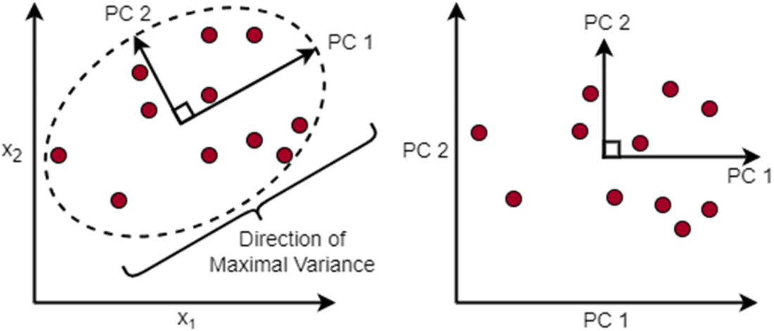
See how PCA rotates the axes and retains the highest-ranked components. section 6.2.3
A practical PCA workflow for molecular descriptors:
- Standardize features when they are on different scales, so their scales are comparable. section 6.2.3
- Choose how many principal components to retain. Different selection criteria can give different answers, and a scree-plot choice can be subjective. section 6.2.3
- Use the reduced representation to support a representative split of molecules for model development. section 6.2 section 6.2.3
Listing 6.6 Representative Data Splitting
def kennard_stone(X, n_samples):
    """Kennard-Stone algorithm for sample selection."""
    n_total_samples = X.shape[0]
    selected_indices = [
        np.argmax(np.sum(distance.cdist(
            X, [X.mean(axis=0)],
            'mahalanobis', VI=np.linalg.inv(np.cov(X.T))
        ), axis=1))
    ]    #A
    remaining_indices = list(range(n_total_samples))
    remaining_indices.remove(selected_indices[0])

    for _ in range(1, n_samples):
        dist_matrix = euclidean_distances(
            X[remaining_indices], X[selected_indices]
        )
        new_index = remaining_indices[
            np.argmax(np.min(dist_matrix, axis=1))
        ]
        selected_indices.append(new_index)
        remaining_indices.remove(new_index)

    return selected_indices

sc = StandardScaler()    #B
pca = PCA(n_components=0.99)

hiv_tar1_lnkd_X = sc.fit_transform(hiv_tar1_lnkd.drop(columns=["lnKD"]))
hiv_tar1_lnkd_X_2D = pca.fit_transform(    #C
    hiv_tar1_lnkd_X    #C
)    #C
lnkd_explained_variance = pca.explained_variance_ratio_    #D

selected_indices_lnkd = kennard_stone(hiv_tar1_lnkd_X_DR, 12)
selected_samples_lnkd = hiv_tar1_lnkd_X_DR[selected_indices_lnkd]

pca.n_components_    #E
>>> 32
selected_indices_lnkd    #F
>>> [25, 3, 47, 10, 21, 5, 42, 39, 26, 18, 35, 24]

lnkd_mask = hiv_tar1_lnkd.index.isin(selected_indices_lnkd)
lnkd_X_test = hiv_tar1_lnkd_X[lnkd_mask]
lnkd_X_train = hiv_tar1_lnkd_X[~lnkd_mask]
lnkd_y_train = hiv_tar1_lnkd["lnKD"][~lnkd_mask]
lnkd_y_test = hiv_tar1_lnkd["lnKD"][lnkd_mask]
Inspect a Python workflow combining StandardScaler, PCA with a 0.99 component setting, and Kennard–Stone sample selection. section 6.2.3
Screening data for drug repurposing
High-throughput screening data can be reduced for visualization to help experts identify promising compounds. One workflow converts molecular SMILES into 2,048-bit Morgan fingerprints with RDKit; optional labels based on a 5 μM IC50 cutoff support additional analysis rather than the unsupervised reduction itself. section 7.1
Other dimensionality reduction approaches include self-organizing maps and uniform manifold approximation and projection (UMAP). section 7.4