A receiver operating characteristic (ROC) curve shows how a classifier behaves as its decision threshold changes. It plots the true-positive rate against the false-positive rate, making the tradeoff between caught positives and false alarms visible. section 8.10
The curve uses two rates calculated from the confusion matrix:
- True-positive rate (TPR) measures true alarms among all relevant instances: TP / (TP + FN). section 8.10
- False-positive rate (FPR) measures false alarms among all irrelevant instances: FP / (FP + TN). section 8.10
- Area under the ROC curve (AUC) summarizes performance across thresholds as one number. section 8.10
Predicting a toddler meltdown
A logistic regression predicts whether a toddler will have a meltdown. Lowering the threshold may catch more meltdowns but create more false alarms; raising it may reduce false alarms while missing more meltdowns. Plotting the ROC curve on held-out test data displays these compromises across thresholds. A tiny dataset can produce an uninformative shape, so the example expands from 25 to 100 samples. section 8.10
Figure 8.8 The receiver operating characteristic (ROC) curve for my logistic regression toddler meltdown prediction, across different thresholds
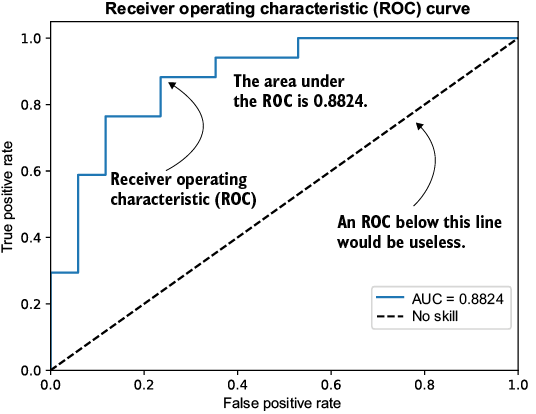
Browse the ROC plot for the toddler-meltdown classifier across different decision thresholds. section 8.10
import numpy as np
import matplotlib.pyplot as plt
from sklearn.linear_model import LogisticRegression
from sklearn.model_selection import train_test_split
from sklearn.metrics import roc_auc_score, roc_curve

x = np.array([0.1, 0.13, 0.22, 0.31, 0.38, 0.38,
             0.46, 0.5, 0.50, 0.56, 0.64, 0.7,
             0.70, 0.85, 0.96, 0.97, 1.06, 1.06,
             1.15, 1.2, 1.2, 1.22, 1.23, 1.24,
             1.31, 1.33, 1.33, 1.41, 1.5, 1.6,
             1.70, 1.78, 1.84, 1.9, 1.90, 1.91,
             1.98, 1.98, 2.03, 2.11, 2.31, 2.37,
             2.42, 2.5, 2.5, 2.50, 2.7, 2.77,
             2.82, 2.92, 3.17, 3.2, 3.28, 3.3,
             3.32, 3.35, 3.46, 3.48, 3.7, 3.77,
             3.8, 3.80, 3.81, 3.82, 3.86, 3.89,
             4.1, 4.20, 4.34, 4.48, 4.49, 4.5,
             4.5, 4.5, 4.63, 4.88, 4.90, 4.96,
             5., 5.07, 5.1, 5.11, 5.15, 5.23,
             5.26, 5.47, 5.6, 5.64, 5.7, 5.73,
             5.81, 5.92, 5.98, 5.99, 6.08, 6.11,
             6.11, 6.2, 6.21, 6.3]) \
   .reshape(-1, 1)  #1


y = np.array([0., 0., 0., 0., 0., 0., 0.,
             0., 0., 0., 0., 0., 0., 0.,
             0., 0., 0., 0.,0., 0., 0.,
             0., 0., 0., 0., 0., 0., 0.,
             0., 0.,0., 0., 1., 0., 0.,
             0.,0., 0., 0., 1.,0., 0.,
             0., 0., 1., 0., 0., 0., 0.,
             0.,1., 0., 1., 1.,1., 0., 0.,
             1., 1., 1.,0., 1., 0., 1., 1.,
             1., 1., 1., 1., 1.,1., 1.,1.,
             1., 1., 1., 1., 1., 0., 1.,1.,
             1., 1., 1., 0., 1., 1., 1., 1.,
             1.,1., 1., 1., 1., 1., 1., 1.,
             1., 1., 1.])  #2


X_train, X_test, Y_train, Y_test = \
    train_test_split(x, y, test_size=1/3)  #3

model = LogisticRegression(penalty=None)  #4
model.fit(X_train, Y_train)  #4

proba = model.predict_proba(X_test)[:, 1]  #5

print(proba)  #6

auc = roc_auc_score(Y_test, proba)  #7
print(f"AUC: {auc:.4f}")  #7


fpr, tpr, thresholds = roc_curve(Y_test, proba)  #8
plt.figure()  #8
plt.plot(fpr, tpr, label=f'AUC = {auc:.4f}')  #8
plt.plot([0, 1], [0, 1], 'k--')  #8
plt.xlim([0.0, 1.0])  #8
plt.ylim([0.0, 1.05])  #8
plt.xlabel('False Positive Rate')  #8
plt.ylabel('True Positive Rate')  #8
plt.title('Receiver Operating '
         'Characteristic (ROC) Curve')  #8

plt.legend(loc="lower right")  #8

plt.show()  #8
Browse the Python listing that computes an ROC curve and ROC AUC with scikit-learn. section 8.10






