Logistic regression is a classifier that gives a soft answer instead of only yes or no. It combines input features with weights and a bias, then turns that result into a score between 0 and 1. Scores near 1 support one class, scores near 0 support the other, and 0.5 marks the decision boundary. section 6.0 section 6.1 section 6.2
Picture a sentiment model: rather than merely calling a sentence happy or sad, it can rate “I’m good” as somewhat happy and a strongly enthusiastic sentence as much closer to 1. A threshold such as 0.5 can then turn the score into a class label, though the score itself keeps useful information about how strongly the model leans. section 6.0 section 6.1
Figure 6.1 Left: The perceptron algorithm trains a discrete perceptron, where the predictions are 0 (happy) and 1 (sad). Right: The logistic regression algorithm trains a continuous perceptron, where the predictions are numbers between 0 and 1 which indicate the predicted level of happiness.
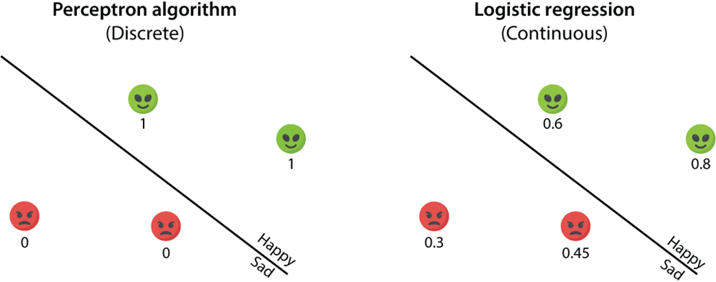
Compare a discrete perceptron with logistic regression: the same separating boundary can produce either hard labels or gradual scores. section 6.1
The calculation has two small steps. First, multiply each feature by its weight, add the results and the bias, and obtain a linear score. Then apply the sigmoid function. Sigmoid squeezes any real-valued score into the interval from 0 to 1: large negative scores approach 0, zero becomes 0.5, and large positive scores approach 1. section 6.11 section 6.2
A tiny word-count prediction
Suppose features count the words “aack” and “beep,” with weights 1 and 2 and bias −4. For a sentence with one “aack” and two “beep” tokens, the linear score is 1×1 + 2×2 − 4 = 1. Applying sigmoid gives 0.731, so the point falls on the side with scores above 0.5. section 6.3
To fit a logistic classifier to labeled data, the algorithm:
- Starts with random weights and a bias. section 6.8
- Picks data points repeatedly and adjusts the weights and bias with the logistic trick. section 6.14 section 6.8
- Uses log loss to measure error; lower total log loss indicates a better fit. section 6.11 section 6.14
For each update, the prediction error is y − ŷ. Each weight changes by a learning-rate-scaled version of that error times its feature value, while the bias changes by the scaled error. Repeating this process moves the boundary toward misclassified points and farther from correctly classified points; over epochs, log loss can fall sharply. section 6.11 section 6.14
Movie-review sentiment
A practical text classifier can turn reviews into word-count features, map positive and negative sentiments to 1 and 0, and train scikit-learn’s LogisticRegression model. Its learned weights can also identify words associated with more positive or negative sentiment. section 6.12
Logistic regression can use any number of features. With two features, its boundary is a line; with more, it is a higher-dimensional hyperplane. For several classes, multiple linear classifiers can be combined with softmax. In practice, mini-batch gradient descent is used instead of updating from one point at a time. section 6.9 section 6.14