A click-or-no-click prediction begins with a probability, not a class label. Logistic regression estimates the probability of a positive binary outcome from one or more predictors. A predetermined decision threshold then turns that probability into a prediction. section 3.3 section 3.3.2
The model first forms a linear predictor, z = β₀ + β₁x₁ + ⋯ + βₖxₖ, where β₀ is the intercept, β₁ through βₖ are coefficients, and x₁ through xₖ are predictors. Unlike a predicted response in linear regression, z represents log-odds: z = log(p/(1 − p)), where p is the probability of the positive outcome. Odds compare the probability of an event with that of its complement; for p = 0.75, the odds are 3 to 1. section 3.3.2
The sigmoid function converts the linear predictor to a probability: p = 1/(1 + e⁻ᶻ). At z = 0, the predicted probability is 0.5. Thus the model combines predictors on the log-odds scale while reporting probabilities between 0 and 1. section 3.3.2
Figure 3.2 The logistic (sigmoid) function maps the linear predictor onto a probability between 0 and 1. The midpoint occurs at 𝑧 = 0, corresponding to a predicted probability of 0.5.
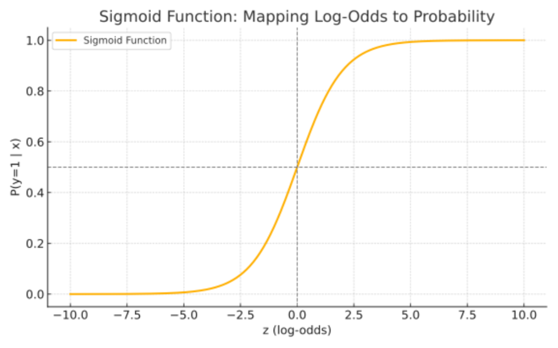
The sigmoid curve shows how the linear predictor maps to probability, with a midpoint at z = 0. section 3.3.2
The coefficients must be estimated from observed outcomes. Maximum likelihood selects coefficient values that give the observed data the greatest support under the model. For observations with outcomes yᵢ and predicted probabilities pᵢ, the likelihood is L(β) = ∏ᵢ pᵢʸⁱ(1 − pᵢ)¹⁻ʸⁱ. The coefficients generally have no closed-form solution, so numerical optimization searches for values that maximize this likelihood. section 3.3.1 section 3.3.2
From predictor to probability
With fitted coefficients β₀ = −6 and β₁ = 1.2, a predictor value of 5 gives z = −6 + 1.2 × 5 = 0 and a predicted probability of 0.50. Values of 2 and 8 give probabilities of approximately 0.027 and 0.973, respectively. section 3.3.2