Adding layers once made some neural networks harder to train rather than better. On CIFAR-10, a plain 56-layer network had higher training error than a plain 20-layer network: extra depth was not automatically useful. The vanishing gradient problem helps explain why early layers in deep networks can fail to learn, though it is not the only obstacle to training them. section 3.1
A network measures the difference between its output and the correct answer as a loss. Backpropagation carries feedback from that loss toward earlier layers, multiplying partial derivatives along the way. When many of those derivatives are smaller than 1, their product shrinks. The earliest layers then receive weight updates too small to support effective learning. Small initial weights can contribute to vanishing gradients; overly large ones can instead produce exploding gradients or saturation. section 2.4 section 3.1
This backward-flow problem is related to, but distinct from, model degradation: information can also become distorted as it travels forward through many layers. Sigmoid and tanh activations compounded the training difficulty by weakening gradients. AlexNet used ReLU activations and careful initialization among several coordinated training choices. ReLU leaves positive inputs unchanged, allowing gradients in that region to pass without repeated reduction; switching from tanh to ReLU accelerated convergence sixfold in an AlexNet experiment. section 3.1 section 2.5.2 section 2.5.5
Figure 2.4 Plot of ReLU (top), sigmoid (middle), and tanh (bottom) activation functions generated in R by the author. Activation functions map input values (on the x-axis) to output values (on the y-axis). For example, ReLU produces 0 for negative inputs; for positive inputs, the output equals the input (0 for x < 0 and linear for x ≥ 0). The sigmoid function maps inputs to values between 0 and 1, resembling an S-curve. Similarly, the tanh function provides a smooth S-shaped curve but maps inputs to values between –1 and 1, centered at 0.
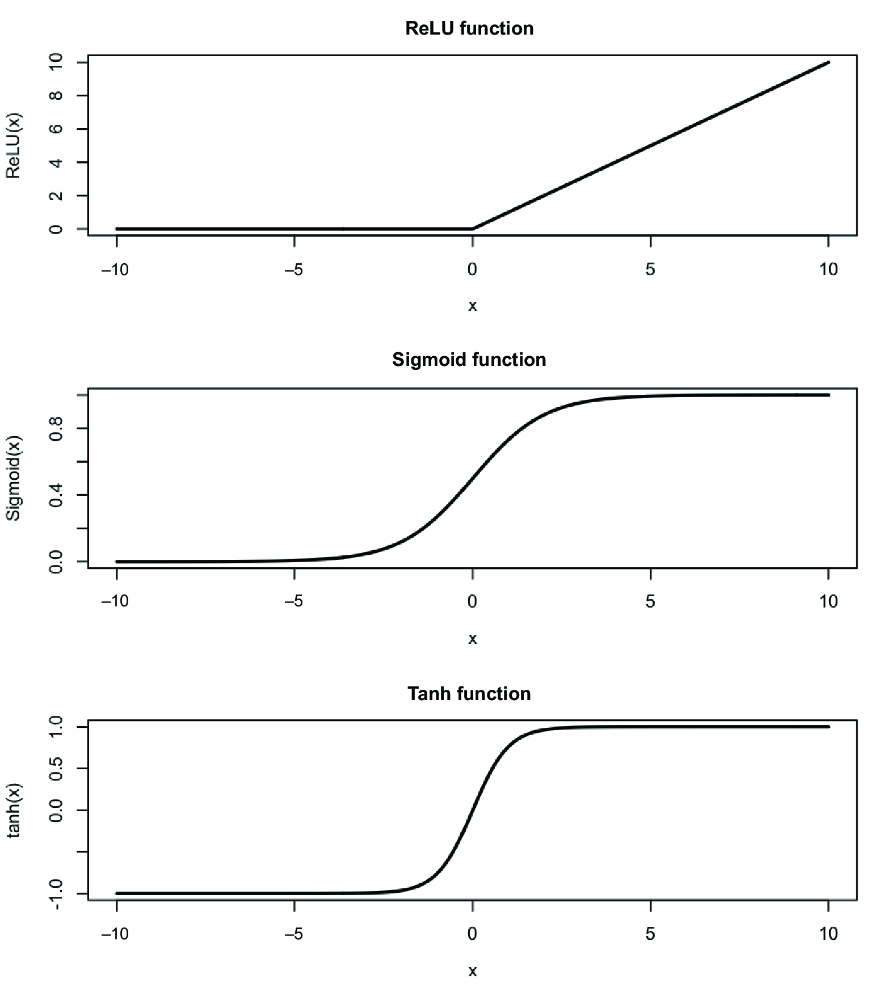
Compare ReLU’s linear positive region with the bounded curves of sigmoid and tanh to see why activation choice matters for gradient flow. section 2.5.2
ReLU and initialization helped make AlexNet practical, but deeper architectures still faced vanishing gradients. Batch normalization and gradient clipping offered partial help without providing a route around dozens of nonlinear layers. ResNet’s shortcut path bypasses transformations and preserves a more direct route for signals. The engineering lesson is that more layers require attention not just to compute, but to how information and training feedback move through the network. section 2.5.5 section 3.1
Figure 3.1 Diagram of a simple ResNet block. It illustrates how input data flows along two paths: one through two transformation layers with activation steps, and another around via a direct “shortcut” path with no transformations. The outputs of these two paths are combined, and the resulting vector undergoes a final activation step. This “shortcut” helps the network learn more effectively by preserving information from earlier layers. Used with permission granted by the lead author (Kaiming He).
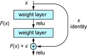
The ResNet block shows an input taking both a transformed path and a direct shortcut path before the two are combined. section 3.1