Kullback–Leibler divergence

As explained in Data Without Labels

Kullback-Leibler divergence is a directed measure of the difference between two probability distributions based on their relative information content.

Kullback–Leibler divergence compares probability distributions by measuring how closely an approximation matches measured or original probabilities. In t-SNE, it compares similarity probabilities from high-dimensional and low-dimensional spaces. section 6.4 section 6.4.1

A KL divergence of zero means the two distributions are identical. The measure therefore supplies the cost that t-SNE seeks to reduce while mapping data into fewer dimensions. section 6.4.1

The t-SNE workflow applies KL divergence after constructing two probability distributions:

• Represent nearby high-dimensional points with high conditional similarity probabilities and distant points with very small probabilities. section 6.4
• Construct low-dimensional probabilities using the Cauchy distribution. section 6.4
• Compare the two distributions and minimize the resulting KL cost function with gradient descent. section 6.4.1

Preserving neighborhood similarity

If two points are nearby in the original space, their conditional similarity probability should remain high in the embedding. KL divergence penalizes differences between those high-dimensional and low-dimensional probabilities. section 6.4 section 6.4.1

Figure 6.13 Comparison of Gaussian distribution vs. Cauchy distribution. (Image source: Quora)

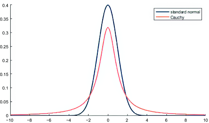
Compare the Gaussian and Cauchy distributions used when forming the high- and low-dimensional probability representations. section 6.4.1

How Data Without Labels covers it

How deep it goes

Defines zero divergence and applies the measure as a gradient-descent cost, without deriving its mathematical formula.

Examples

Uses conditional similarities for nearby and distant points, plus Gaussian-versus-Cauchy distribution comparisons.

What it assumes

Assumes probability distributions and connects optimization through gradient descent with earlier multidimensional scaling treatment.

What you can do after

Evaluate how closely low-dimensional similarity probabilities match high-dimensional probabilities in t-SNE.

How it connects

Connects probability distributions, t-SNE, SNE, Gaussian distribution, Cauchy distribution, MDS, and gradient descent.

liveBookmanning.com

Read Data Without Labels on liveBook Get the book at manning.com

Also explained in

• 

  liveBookmanning.com
  Reinforcement Learning from Human FeedbackForward KL divergence is KL divergence from a target distribution to an approximating distribution, with expectation taken under the target distribution.
• 

  liveBookmanning.com
  Graph Neural Networks in ActionA measure of the difference between two probability distributions, quantifying the information cost of approximating one with another.
• 

  liveBookmanning.com
  Math and Architectures of Deep LearningA loss term based on Kullback-Leibler divergence that penalizes differences between probability distributions, such as an encoder's latent distribution and a chosen prior.
• 

  liveBookmanning.com
  Learn Generative AI with PyTorchA divergence measure used as a regularization term to encourage a latent-variable distribution to resemble a normal distribution.
• 

  liveBookmanning.com
  Build a Reasoning Model (From Scratch)A measure of how different two probability distributions are, used here for soft distillation.
• 

  liveBookmanning.com
  Machine Learning Algorithms in DepthKullback-Leibler divergence is a nonnegative measure of the discrepancy between two probability distributions.
• 

  liveBookmanning.com
  Evolutionary Deep Learning: Genetic algorithms and neural networksA divergence-based measure comparing probability distributions through differences in their information content.
• 

  liveBookmanning.com
  Causal AIKullback–Leibler divergence quantifies the difference between two probability distributions.
• 

  liveBookmanning.com
  Bayesian Optimization in ActionKullback–Leibler divergence is a nonnegative statistical divergence that quantifies how one probability distribution differs from another.
• 

  liveBookmanning.com
  Optimization Algorithms: AI techniques for design, planning, and control problemsKullback–Leibler divergence is a metric quantifying the dissimilarity between two probability distributions.
• 

  liveBookmanning.com
  Deep Learning with R, Third EditionKullback–Leibler divergence is a measure of how one probability distribution differs from a reference probability distribution.

Compare how 12 books explain Kullback–Leibler divergence →

Related concepts

• Group Relative Policy Optimizationpart of · Group Relative Policy Optimization is a reinforcement-learning algorithm that updates a policy using relative rewards or advantages estimated from groups of sampled outputs or actions.
• t-SNEused by · t-SNE is a nonlinear dimensionality-reduction technique that maps high-dimensional data to a lower-dimensional space while emphasizing local similarities or neighborhood relationships.
• variational inferenceused by · Variational inference is an approximate inference technique that optimizes a tractable family of probability distributions to approximate a target distribution, often a posterior.
• variational Gaussian processused by · A variational Gaussian process is a scalable approximation to a Gaussian process whose posterior is represented through variational inference over a finite set of inducing points.

This explainer was generated by Manning's knowledge graph from the text of Data Without Labels. The section links point to the parts of the book it draws on.