Kullback–Leibler divergence

As explained in Machine Learning Algorithms in Depth

Kullback-Leibler divergence is a nonnegative measure of the discrepancy between two probability distributions.

Kullback–Leibler (KL) divergence measures the discrepancy between probability distributions. In variational inference, p(x) is a target posterior and q(x) is a tractable approximation with adjustable parameters. Minimizing their divergence turns posterior approximation into an optimization problem. section 1.4.1

Direction matters. Reverse KL is KL(q||p) = E_q[log(q(x)/p(x))]; forward KL is KL(p||q) = E_p[log(p(x)/q(x))]. Both are nonnegative, but exchanging p and q can change the preferred approximation. When a single-peaked q approximates a two-peaked p, reverse KL tends to concentrate on one mode, while forward KL can favor a broader fit covering both peaks. section 3.1 section 1.4.1

Check the Gaussian objective

Let p(x) = N(0,1) and q(x) = N(μ,σ²). Computing reverse KL gives KL(q||p) = (μ² + σ² − 1 − log σ²)/2. Fixing σ² = 4 reduces this to (μ² + 3 − log 4)/2. Its minimum over μ is at μ = 0: matching the means helps, but the divergence remains positive because the variances differ. section 3.1

Figure 3.2 Forward KL (left) q(x) overestimates the support, while reverse KL (right) q(x) locks onto a mode.

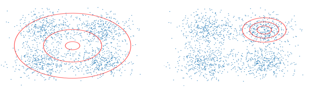
Compare the broad forward-KL approximation with the reverse-KL approximation concentrated on one mode of the target. section 3.1

The same discrepancy serves several objectives. In variational inference it contributes to a variational free-energy objective and the derivation of a bound used for optimization. A KL-based bound also supports iterative mutual-information maximization. In a time-series LSTM-VAE, minimizing KL structures the latent Gaussian toward N(0,1), alongside a likelihood objective for detecting anomalies. section 3.1 section 3.4 section 11.1.1

How Machine Learning Algorithms in Depth covers it

How deep it goes

Defines directional KL, works through Gaussian parameters, and relates its penalty to variational free energy and optimization.

Examples

Uses Gaussian approximations, a two-mode target, a wireless channel, and an LSTM-VAE anomaly detector.

What it assumes

Assumes familiarity with probability distributions and Gaussian parameters while introducing tractable posterior approximation.

What you can do after

Evaluate/understand directional approximation behavior and compute KL divergence for two univariate Gaussians as an exercise.

How it connects

Connects to variational inference, variational free energy, mutual information, and variational autoencoders.

liveBookmanning.com

Read Machine Learning Algorithms in Depth on liveBook Get the book at manning.com

Also explained in

• 

  liveBookmanning.com
  Reinforcement Learning from Human FeedbackForward KL divergence is KL divergence from a target distribution to an approximating distribution, with expectation taken under the target distribution.
• 

  liveBookmanning.com
  Graph Neural Networks in ActionA measure of the difference between two probability distributions, quantifying the information cost of approximating one with another.
• 

  liveBookmanning.com
  Math and Architectures of Deep LearningA loss term based on Kullback-Leibler divergence that penalizes differences between probability distributions, such as an encoder's latent distribution and a chosen prior.
• 

  liveBookmanning.com
  Learn Generative AI with PyTorchA divergence measure used as a regularization term to encourage a latent-variable distribution to resemble a normal distribution.
• 

  liveBookmanning.com
  Build a Reasoning Model (From Scratch)A measure of how different two probability distributions are, used here for soft distillation.
• 

  liveBookmanning.com
  Evolutionary Deep Learning: Genetic algorithms and neural networksA divergence-based measure comparing probability distributions through differences in their information content.
• 

  liveBookmanning.com
  Causal AIKullback–Leibler divergence quantifies the difference between two probability distributions.
• 

  liveBookmanning.com
  Data Without LabelsKullback-Leibler divergence is a directed measure of the difference between two probability distributions based on their relative information content.
• 

  liveBookmanning.com
  Bayesian Optimization in ActionKullback–Leibler divergence is a nonnegative statistical divergence that quantifies how one probability distribution differs from another.
• 

  liveBookmanning.com
  Optimization Algorithms: AI techniques for design, planning, and control problemsKullback–Leibler divergence is a metric quantifying the dissimilarity between two probability distributions.
• 

  liveBookmanning.com
  Deep Learning with R, Third EditionKullback–Leibler divergence is a measure of how one probability distribution differs from a reference probability distribution.

Compare how 12 books explain Kullback–Leibler divergence →

Related concepts

• Group Relative Policy Optimizationpart of · Group Relative Policy Optimization is a reinforcement-learning algorithm that updates a policy using relative rewards or advantages estimated from groups of sampled outputs or actions.
• t-SNEused by · t-SNE is a nonlinear dimensionality-reduction technique that maps high-dimensional data to a lower-dimensional space while emphasizing local similarities or neighborhood relationships.
• variational inferenceused by · Variational inference is an approximate inference technique that optimizes a tractable family of probability distributions to approximate a target distribution, often a posterior.
• variational Gaussian processused by · A variational Gaussian process is a scalable approximation to a Gaussian process whose posterior is represented through variational inference over a finite set of inducing points.

This explainer was generated by Manning's knowledge graph from the text of Machine Learning Algorithms in Depth. The section links point to the parts of the book it draws on.