Kullback–Leibler divergence (KL divergence, KLD) measures the dissimilarity between two probability distributions. It removes the baseline offset in cross-entropy: cross-entropy between identical distributions equals their entropy, whereas KL divergence is zero when they are identical. In classification, minimizing cross-entropy against a fixed ground-truth distribution is therefore equivalent to minimizing KL divergence. section 6.4
KL divergence compares how one distribution assigns probability mass relative to another. Its logarithmic ratio gives positive contributions where the first distribution assigns more probability than the second and negative contributions where it assigns less; weighting by the first distribution makes the total nonnegative. It is zero only for identical distributions, and it is directed: D(X1, X2) need not equal D(X2, X1). section 6.4
Comparing Gaussian distributions
For univariate and multivariate Gaussians, KL divergence has closed-form expressions. Distributions with closer spreads produce lower divergence in a comparison with equal means; distributions with closer locations produce lower divergence in a comparison with equal spreads. PyTorch provides torch.distributions.kl_divergence for computing these comparisons. section 6.4.1
In a variational autoencoder (VAE), the encoder emits a latent distribution for each input, commonly a Gaussian with mean and covariance. Training minimizes reconstruction loss plus a weighted KL-divergence loss between that encoder distribution and a fixed prior, usually a zero-mean, unit-covariance Gaussian. The added term regularizes the latent space rather than merely seeking accurate reconstruction. section 14.7.2 section 14.7
Matching the standard Gaussian favors a compact, smooth latent space: latent vectors are restrained from spreading broadly and are concentrated mostly within a unit ball. With a diagonal covariance assumption, the Gaussian KL term is minimized when the encoder mean is at the origin and each variance is one. This regularization distinguishes a VAE’s latent space from an autoencoder trained only for reconstruction. section 14.7.7 section 14.6
Figure 14.10 The difference between the learned latent spaces of the autoencoder and VAE. We train an autoencoder and a VAE with nz = 2 on MNIST and plot the latent space for the test set. Autoencoders only minimize the reconstruction loss, so any latent space is equally acceptable as long as the reconstruction loss is low. As expected, the learned latent space is sparse and has a very high spread. VAEs, in contrast, minimize reconstruction loss with regularization. This is done by minimizing the KL divergence between the learned latent space and a known prior distribution 𝒩( , I). Adding this regularization term ensures that the latent space is constrained within a unit ball. This can be seen in figure 14.10b, where the learned latent space is much more compact.
|
(a) Autoencoder latent space nz=2) |
|
(b) VAE latent space (nz=2) |
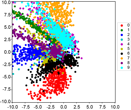
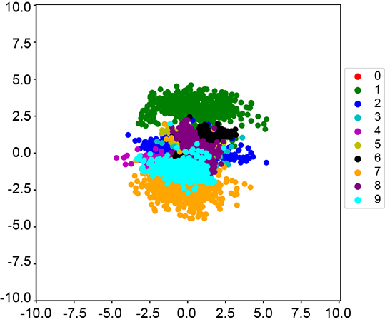
Compare the sparse, widely spread autoencoder latent space with the compact VAE latent space produced by reconstruction plus KL regularization. section 14.7.8