Kullback–Leibler (KL) divergence measures how far one probability distribution is from an expected distribution. In a variational autoencoder (VAE), it is a regularization term: it penalizes the encoder when its learned latent distribution departs from a standard normal distribution. section 7.3.1
A conventional autoencoder encodes an input as a point and minimizes reconstruction loss. A VAE encodes an input as a distribution and minimizes reconstruction loss plus KL divergence. The first term rewards faithful images; the second encourages latent representations that do not simply memorize the training images. section 7.0 section 7.3.1
Training on face images
For each 3 × 256 × 256 face image, the encoder produces means and standard deviations for a 100-dimensional latent representation. A sampled encoding goes to the decoder, which reconstructs the image. Training adds pixel-level reconstruction loss to KL divergence and backpropagates the total. Under the assumed normal distribution, KL divergence is summed across the 100 dimensions; it is zero when their means are 0 and standard deviations are 1, and greater than zero otherwise. section 7.3.1 section 7.3.2
Figure 7.6 The architecture of a VAE and the steps to train one to generate human face images. A VAE consists of an encoder (middle upper left) and a decoder (middle bottom right). In each iteration of training, human face images are fed to the encoder (step 1). The encoder compresses the images to probabilistic points in the latent space (step 2; since we assume normal distributions, each probability point is characterized by a vector of means and a vector of standard deviations). We then sample encodings from the distribution and present them to the decoder. The decoder takes sampled encodings (step 3) and reconstructs images (step 4). The VAE adjusts its parameters to minimize the sum of reconstruction loss and the KL divergence. The KL divergence measures the difference between the encoder’s output and a standard normal distribution.
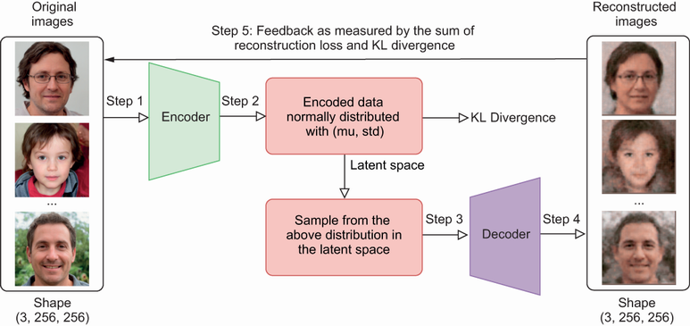
Follow the encoder, latent sampling, decoder, and combined loss through one VAE training iteration. section 7.3.2
The practical payoff is a more structured latent space. After training, encodings can be sampled to generate new faces or combined to explore image features. For example, averaging encodings within face-image groups makes it possible to perform encoding arithmetic and decode the result. KL divergence encourages that structure; it is not itself the arithmetic operation. section 7.3.2 section 7.4.4