Kullback–Leibler (KL) divergence measures how different an approximating distribution q is from a target distribution p. In variational inference, q approximates the posterior p(θ | D). KL divergence is nonnegative, equals zero when the distributions match, and grows when q assigns probability where p assigns little. section 6.4
Use these properties to interpret the optimization:
- Treat the divergence as directional: the approximation q is evaluated against the target p, so disagreement is weighted according to q. section 6.4 section 6.15
- Expect high values when q places substantial density in regions where p has little density. section 6.4
- Minimize KL divergence by maximizing the evidence lower bound (ELBO), typically through gradient-based optimization. section 6.6 section 6.15
Shaping a balloon around jelly
Imagine shaping a balloon to cover jelly spread across a table. If the balloon spends much of its area outside the jelly, the wasted area represents a poor approximation and a larger KL divergence. If it follows the jelly closely, the divergence approaches zero. section 6.4
Optimizing a Beta approximation
During optimization, gradient descent adjusts q’s mean and spread toward a target Beta distribution. As the ELBO rises, KL divergence falls; after convergence, q can stand in for the true posterior in Bayesian inference. section 6.6
Figure 6.2 The KL divergence is large when the approximating distribution 𝑞 yields high density where 𝑝 is small. When the two distributions match, the KL divergence decreases to be close to 0.
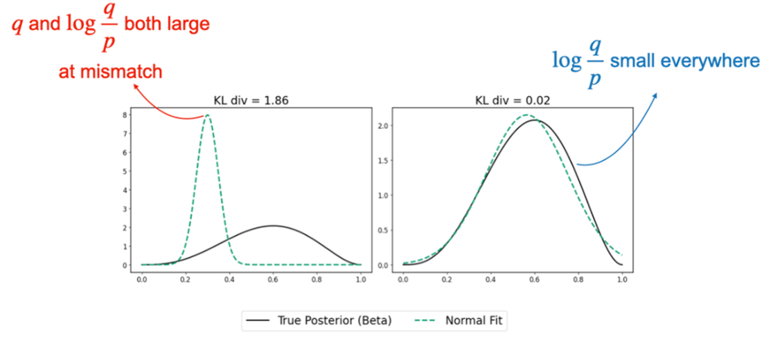
Visualizes why KL divergence grows when q assigns high density where p is small and shrinks when the distributions match. section 6.4