A latent space is a learned vector space for representing data. Instead of working directly with words or image pixels, a model works with points in this space. Their positions can capture useful relationships: similar words may lie near one another, while a point in an image latent space can be decoded into a picture. What the space captures depends on the data and the task. section 14.5.2 section 14.5.3 section 17.1.1
Four words on a map
Imagine placing “cat,” “dog,” “wolf,” and “tiger” on a two-dimensional plane. One direction could take you from pet to wild animal; another could take you from canine to feline. Real word embeddings use many more dimensions, but the idea is the same: distances and directions can express relationships learned from data. They are not a universal map of language. section 14.5.2 section 14.5.3
An embedding layer is a practical way to learn such a space. It looks up each integer token ID and returns a dense vector. For a batch of sequences, its output has shape `(batch_size, sequence_length, embedding_size)`. The vectors start at random positions and are adjusted by backpropagation as the model trains. Unlike one-hot vectors, these representations are dense and relatively low-dimensional. section 14.5.2 section 14.5.3
Put embeddings into a text model
In R/Keras, `layer_embedding(input_dim = max_tokens, output_dim = 64L, mask_zero = TRUE)` turns integer-indexed tokens into 64-value vectors before a bidirectional LSTM processes the sequence. The embedding space is learned for the model’s task; a movie-review sentiment model need not organize words exactly as a legal-document classifier would. section 14.5.3
Latent spaces also make generation possible. An image generator, or decoder, maps a latent point back to pixels. After learning a suitable space, you can sample new points and decode images not present in the training set. In a variational autoencoder (VAE), an encoder maps an image to parameters of a distribution over latent points; a sampled point is then passed to the decoder. section 17.1.1 section 17.1.2
Walk through handwritten digits
A VAE trained on MNIST digits uses a two-dimensional latent space. After training, make a grid of points with `z <- seq(-1, 1, length.out = 30)` and `z_grid <- as.matrix(expand.grid(z, z))`, then obtain images with `predict(vae$decoder, z_grid, verbose = 0)`. Arranging the decoded digits in the same grid lets you see how the output changes across the space. section 17.1.3
Figure 17.5 Grid of digits decoded from the latent space
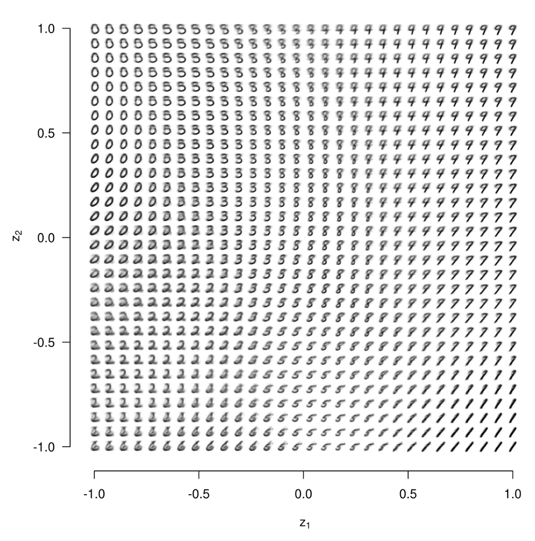
The grid makes the two-dimensional example tangible: each position is a latent point decoded into a digit image. section 17.1.3
Choose the space for the job. More dimensions give a model room to learn more complex representations, but increase computation and can encourage unwanted patterns. VAEs offer structured, continuous image representations useful for editing and animation; diffusion models are favored for realistic image generation. Neither a convincing image nor a meaningful vector direction means the model has learned a consistent understanding of the physical world. section 4.1.3 section 17.1.1 section 17.4