A latent space is a learned transformed space in which each input is represented by a latent vector, or embedding. The representation retains features useful for an objective while discarding other information, and it is typically lower-dimensional than the observed input. Learning the mapping forces a limited-size vector to preserve what matters most. section 14.0
Geometrically, latent-space modeling learns a manifold around inputs sharing a property of interest. Encoding projects an input onto that manifold: the in-manifold component becomes the embedding, while the orthogonal component is discarded as information unrelated to the property, such as image background. section 14.1 section 14.8
Figure 14.1 Two examples of latent subspaces, with planar and curved manifolds, respectively. The solid line shows the latent vector, and the dashed line represents the information lost by projecting onto the latent subspace.
|
(a) Planar latent subspaces |
|
(b) Curved latent subspace |
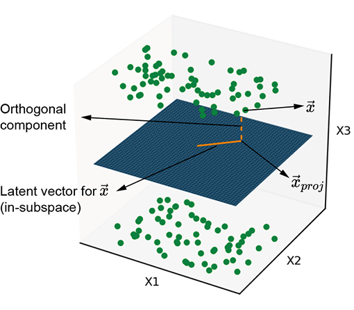
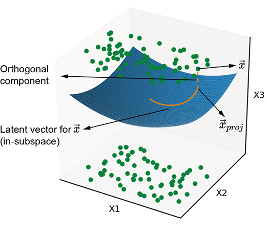
Compare planar and curved manifolds to see a latent vector as a projection and the dashed component as discarded information. section 14.1
A useful latent representation can provide:
- A compact, less noisy representation focused on discriminative information. section 14.3
- A friendlier coordinate system for a downstream task; mapping Cartesian points to polar coordinates turns a circular boundary into the linear rule r = a. section 14.3
- Similarity estimates from Euclidean distances between latent vectors. section 14.3
- Generative class probabilities rather than only a thresholded class decision. section 14.2
PCA is a linear instance of latent-space modeling: its manifold is a best-fit hyperplane. Autoencoders generalize this idea with nonlinear encoder and decoder networks. The encoder maps an input to a size-constrained latent vector; the decoder reconstructs the input. End-to-end training minimizes reconstruction loss, so no labels are required. section 14.5 section 14.8
Figure 14.5 Schematic representation of an autoencoder. The encoder transforms input into a latent vector. The decoder transforms the latent vector into reconstructed input. We minimize the reconstruction loss—the distance between the reconstructed input and the original input.
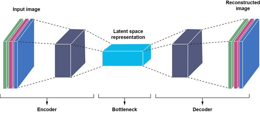
The encoder–decoder diagram makes the information bottleneck and reconstruction-loss objective explicit. section 14.5
Low reconstruction error alone does not ensure a useful geometry: both smooth and zigzag manifolds can reconstruct training points well. Regularization favors compact, smooth spaces where comparable input distances remain more consistent after projection. A variational autoencoder (VAE) adds KL-divergence loss that draws encoder-produced latent distributions toward a chosen prior, commonly a zero-mean unit-covariance Gaussian. section 14.6 section 14.7.2 section 14.7.7
Unlike a standard autoencoder’s direct encoding, a VAE encoder emits distribution parameters and samples a latent vector during training; at inference it uses the emitted mean. Nearby sampled latent points must decode to nearby input regions, promoting smoothness. The decoder maps latent points back toward reconstructed inputs. section 14.7.1 section 14.7.4
MNIST: autoencoder versus VAE
With a two-dimensional latent space, an autoencoder trained only on reconstruction can learn a sparse, widely spread representation. A VAE combines reconstruction with KL regularization toward N(0, I), yielding a more compact latent space while reconstructing digit images. section 14.7.8
Figure 14.10 The difference between the learned latent spaces of the autoencoder and VAE. We train an autoencoder and a VAE with nz = 2 on MNIST and plot the latent space for the test set. Autoencoders only minimize the reconstruction loss, so any latent space is equally acceptable as long as the reconstruction loss is low. As expected, the learned latent space is sparse and has a very high spread. VAEs, in contrast, minimize reconstruction loss with regularization. This is done by minimizing the KL divergence between the learned latent space and a known prior distribution 𝒩( , I). Adding this regularization term ensures that the latent space is constrained within a unit ball. This can be seen in figure 14.10b, where the learned latent space is much more compact.
|
(a) Autoencoder latent space nz=2) |
|
(b) VAE latent space (nz=2) |
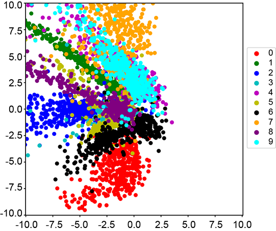
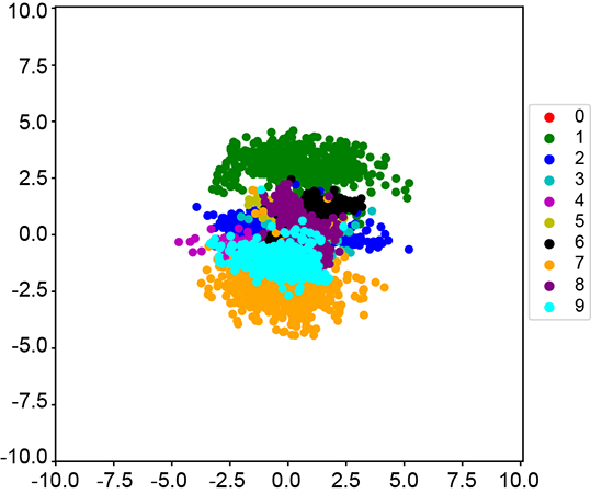
The two-dimensional MNIST plots contrast an unregularized autoencoder space with the VAE’s compact, prior-constrained space. section 14.7.8