Variance measures how spread out values are around their mean. It captures typical squared deviation, rather than merely the range between minimum and maximum values: a few distant extremes need not make an otherwise tightly packed collection broadly spread. For a random variable X with mean μ, var(X) = E((X − μ)²) = E(X²) − E(X)². Small variance means likely values cluster near μ; large variance means they lie farther away. Standard deviation is the square root of variance. section 5.7.2
Figure 4.2 A 1D distribution of points. The distance between extreme points is not a fair representation of the spread of points: the distribution is not uniform, and the extreme points are far from the others. Most points are within a more tightly packed region.
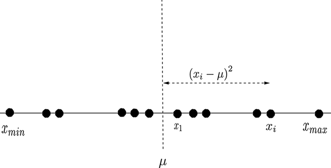
A point cloud can have distant extremes while most points remain close together, so range alone is a poor measure of its typical spread. section 4.4
For a finite sample, first compute its mean, then average the squared distances of sample values from that mean. When the population distribution is known, its variance may have a closed-form expression; when it is unknown, sample variance summarizes the sampled point cloud. Larger variance relative to the mean generally requires more samples for a sample average to closely approximate the expected value. section 5.8 section 5.7.2
In multiple dimensions, spread depends on direction, so there is no single scalar variance for the whole point cloud. The covariance matrix C represents directional spread. Along a unit direction l̂, variance is the quadratic form l̂ᵀCl̂. Its maximum occurs at C’s eigenvector with the largest eigenvalue; that direction is the first principal axis, and the eigenvalue is its principal variance. section 4.4.1 section 4.7
Variance supports common machine-learning decisions:
- Retain high-variance principal directions while treating low-variance directions as possible noise for dimensionality reduction. section 4.7
- Parameterize probability distributions, whose mean and variance describe location and spread. section 5.7
- Fit Gaussian models with sample mean and sample variance or covariance under maximum likelihood estimation. section 6.10
- Represent a VAE encoder output as a Gaussian whose small covariance produces a tight latent sample cluster. section 14.7.1
Estimating variance from sampled distributions
A PyTorch distribution exposes both a theoretical variance and sampled values. Draw many samples, compute samples.var(), and compare it with dist.variance. This is illustrated for Bernoulli, binomial, and Gaussian distributions; the sample statistic approaches the distribution property with sufficiently many samples. For a Gaussian, increasing σ produces a wider, lower bell shape because total probability remains one. section 5.9.5 section 5.9.2 section 5.9.3